
DATA RELIABILITY AND DATA SELECTION
IN REAL TIME HIGH FIDELITY SENSOR NETWORKS
Nina Peterson
Department of Natural Sciences and Mathematics, Lewis-Clark State College, Lewiston, Idaho, U.S.A.
Behrooz A. Shirazi, Medha Bhadkamkar
School of Electrical Engineering and Computer Science, Washington State University, Pullman, Washington, U.S.A.
Keywords: Data quality, Data selection, Wireless sensor networks, Bayesian network, Knapsack optimization.
Abstract: Due to advances in technology, sensors in resource constrained wireless sensor networks are now capable of
continuously monitoring and collecting high fidelity data. However, all the data cannot be trusted since data
can be corrupted due to several reasons such as unreliable, faulty wireless sensors or harsh ambient
conditions. Further, due to bandwidth constraints that limit the amount of data being transmitted in sensor
networks, it is important that only the high priority, accurate data is transmitted. In this paper, we propose a
data selection model that makes two significant contributions. First, it provides a way to determine the
confidence in or reliability of the data values and second, it determines which subset of data is of the highest
quality or of most interest given the state of the network system and its current available bandwidth. Our
model is comprised of two phases. In Phase I we determine the reliability of each input data stream using a
Bayesian network. In Phase II, we use a 0-1 Knapsack optimization approach to choose the optimal subset
of data. An evaluation of our best data selection model reveals that it eliminates erroneous data and
accurately determines the subset of data with the highest quality when compared with conventional
algorithms.
1 INTRODUCTION
There is an increasing demand for high fidelity,
continuous data sampling from resource constrained
wireless sensor network environments. For instance,
real-time applications that monitor environments,
such as an active volcano, employ wireless sensor
networks to continuously monitor, collect and
analyze data under extreme environmental
conditions such as snow, wind, rain or ice. Ideally,
we should be able to collect and transmit all this data
continuously. However, in the real world, this is not
feasible since the continuously sampled data is of
such high frequency and resolution that it can
quickly consume all the available bandwidth and
drop data packets during transmission. Additionally,
due to sensor malfunctions and harsh environmental
conditions, the quality of data cannot be trusted at all
times. Thus, it is imperative that only the high
quality data is transmitted over the network, and the
remaining data is transmitted only if bandwidth
space permits. The quality of data for any wireless
sensor network deployment is an important issue
that has ramifications in network management and is
of significance to the user. Dynamic scheduling
algorithms, such as Tiny-DWFQ (Peterson et al.,
2008), are complementary to this work and may be
utilized to assign priorities to the data to ensure that
high quality data would be made available to the end
users.
This paper presents a two-phase, best data
selection model that determines the best subset of
data to select from a given set of input data streams
in a sensor network. Phase I identifies reliable data
from different input data streams, while Phase II
selects the best data subset for delivery to the end
user given the network bandwidth. We applied our
model to the data collected by a volcanic monitoring
sensor network (called OASIS) deployed at Mount
St. Helens, an active volcano site. The sensors in
OASIS collect and transmit hi-fidelity data in real
time which may be prone to errors and hence
42
Peterson N., A. Shirazi B. and Bhadkamkar M. (2011).
DATA RELIABILITY AND DATA SELECTION IN REAL TIME HIGH FIDELITY SENSOR NETWORKS .
In Proceedings of the 1st International Conference on Pervasive and Embedded Computing and Communication Systems, pages 42-53
DOI: 10.5220/0003365600420053
Copyright
c
SciTePress

provides an ideal framework for the evaluation for
our model. Our results reveal that our model
determines the most appropriate subset of data with
high accuracy.
The rest of the paper is organized as follows.
Section 2 discusses the motivations for and
contributions of the project. To elucidate our setup,
we present relevant background information in
Section 3. Details of each phase of our model
including our solutions to relevant challenging
issues they posed are discussed in Section 4. We
present our analysis and evaluation of the proposed
system in Section 5 and make concluding remarks in
Section 6.
2 MOTIVATIONS
AND CONTRIBUTIONS
Our motivation for developing the optimal data
selection model was due to the lack of an acceptable
existing solution. Our investigation revealed that
amongst the researchers who addressed optimal data
selection, there were three common shortcomings
that degraded the overall performance of the system.
In this section, we discuss each of these
shortcomings and how we address them in our
optimal data selection model. Our solution enables
us to achieve an overall enhanced accuracy.
2.1 Improving Data Confidence
and Assignment
The first issue we observed in the existing solutions
was the method in which the data confidence levels
(reliabilities) were assigned. We define the data
confidence level as the assurance or belief that the
data value we obtained is correct when compared to
the true value. It is a measure of the reliability of the
data and is a crucial parameter in several studies.
In previous work for optimal data selection in
wireless sensor networks, the user assigned a
confidence level to each type of data or each
individual parameter using either expert knowledge
(Lee and Meier, 2007) (Kumar, et al., 2003) or a
very simplistic metric such as ranking or thresholds
(Ahmen et al., 2005) (Bettini et al., 2007). While
both expert knowledge and user-defined threshold
values have an impact on the confidence level of the
data, we believe that these methods are only reliable
in extremely simplistic situations and environments.
For example, if the threshold method was used to
determine the “hotness” inside a building, a
threshold of 75°F would be reasonable, given the
criteria. However, in several sophisticated scenarios,
such as our volcanic activity monitoring scenario,
numerous factors and complex conditions affect the
data values continuously and using non-adaptive
threshold values to assign data confidence levels can
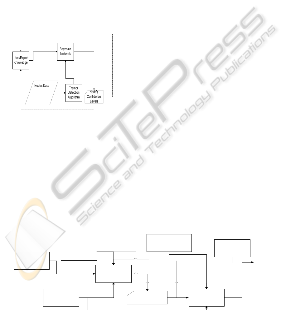
produce inaccurate results. Hence, we developed an
adaptive optimized confidence level mechanism
using a Bayesian Network as shown in Figure 1. The
Bayesian Network minimizes the effects of users’
(expert) knowledge imperfections and allows us to
render a dynamic confidence level to each data flow.
Our Bayesian network uses both expert knowledge
and node data as the input parameters. Using this
input, the Bayesian network is able to determine the
confidence level of the node’s data. This is further
discussed in detail in Section IV. Before passing the
raw data into the Bayesian network we first run it
through a tremor detection algorithm. The tremor
detection algorithm is the industry standard that is
used for determining the possibility of seismic
activity.
2.2 Dynamic Confidence Assignments
Existing confidence value assignments mechanisms
are generally static and do not change through the
lifetime of the network (Bettini et al., 2009). We
believe that it is unrealistic to assume that the
reliability of sensors and their readings do not
change (possibly drastically) throughout the lifetime
of the network. For example, let us assume that
shortly after deployment, node X recorded accurate
seismic data and was assigned a corresponding
confidence level of 98%. However, a minor eruption
(or rock fall) caused severe damage to the antenna
for node X, resulting in bad readings. In this
scenario, it would be damaging to the network to
continue to represent node X’s seismic reading with
a confidence level of 98%.
To adapt to the continually changing state of the
network, we designed our confidence level
assignment to be dynamic, where the Bayesian
network re-computes the confidence level for each
data stream after a certain, application specific, time
period (say every 5 minutes). The user can also
execute a re-computation if necessary.
The dynamic confidence assignment also reduces
the impact of any errors that result from the user’s
input to the system. While we do not believe that the
user knowledge or a threshold should be the sole
criteria for determining the confidence level, to
some degree this information must be inserted into
the model. Thus, we use this information as a
DATA RELIABILITY AND DATA SELECTION IN REAL TIME HIGH FIDELITY SENSOR NETWORKS
43
starting point and continually update and adjust the
confidence level to minimize any errors in these
values. The Bayesian Network allows us to render a
dynamic confidence level to each data flow. We
choose to use a Bayesian network for two reasons.
First, it has an inherent ability to minimize
inaccuracies within the system. For example, if one
of the parameters, say y has an initial probability of
q, any errors in the assignment of q are minimized
by the other variables and their relationships within
the network. This property of Bayesian networks can
be seen in the ability of the user to assign equal,
random or normalized probabilities to variables to
which an initial probability is unknown.
Figure 1: Adaptive Optimized Confidence Level.
Secondly, Bayesian networks do not require all
the possible outcomes to be expressed. In order to
express all outcomes, extensive knowledge of all
possible actions that may occur must be known. This
is fine for a very controlled and simplistic scenario;
however our real world volcanic scenario makes this
assumption impractical, if not impossible.
2.3 Optimal Subset Selection
In our investigation of the current context modelling
techniques developed for wireless sensor networks,
it appears that none of them address the optimal
subset selection problem. Optimal subset selection
has been studied and proven to be beneficial in many
other areas of research since it allows one to inject
the best possible subset of data in the network to
maximize one’s return.
In order to choose the optimal subset of data, we
utilized a 0-1 Knapsack approach. This enabled us to
maximize the return (in our case value or priority of
the data) while minimizing the cost (in our case cost
of transmission in terms of bandwidth). This ensures
that data with a low confidence (say 5%) does not
degrade the network performance as it could in the
general models. It should be noted that cluster data
is used as an input to the Bayesian network, as
shown in Figure 2, in order to both provide a way to
validate the data of closely placed nodes
(geographically) and to be able to provide a way to
identify areas of activity. A cluster is a group of
neighboring sensor nodes whose data are correlated
to determine the occurrence of an event (such as a
tremor in the context of volcano monitoring).
The quality of the data which is the output of
Phase I, the current data priority and the network
bandwidth are input to Phase II. The current data
priority is an adaptive measure of the importance of
a specific data type. Like the seismic data reliability,
the seismic data priority is also derived from Phase
I. The Bayesian network does not directly determine
the occurrence of a tremor. However, the occurrence
of a tremor directly affects the rest of the network
that it was a part of. We choose to utilize this in
order to assign a seismic data priority to each data
flow. This allowed us to give more importance to
nodes in area(s) where we believe activity (seismic
tremor) is occurring. This is very important as we
are not just interested in the most reliable data but
rather in the most important, reliable data. Thus we
combine (through a summation) the seismic data
reliability and the seismic data priority into one
entity, the confidence parameter, vi. This is
discussed in detail in Section 4.
Figure 2: Optimal Data Selection.
U se r/E xp e rt
Input
Bayesian
Network
Q uality of
Data
Updates baseline confidence
Cluster Data
0-1
Knapsack
O p tim a l d a ta su b s e t
Nodes Data
Bandw idth
R esources
C u rre n t D a ta
Priority
PECCS 2011 - International Conference on Pervasive and Embedded Computing and Communication Systems
44

3 BACKGROUND
INFORMATION
3.1 OASIS
In this section, we provide an overview of the
Optimized Autonomous Space In-Situ Sensor-web
(OASIS) (Song et al., 2008), which provides the
testbed for the design and development of our data
selection model. While volcanic sensor-webs used in
previous studies were deployed only for a few
weeks, OASIS is the first volcanic monitoring
sensor network deployment which has been
deployed for over a year at the volcano site at Mount
St. Helens. The OASIS wireless sensor network is
composed of several Imote2 sensor nodes deployed
on Mount St. Helens. Each node is attached to a
seismic sensor, an infrasonic sensor, and a lightning
sensor. To withstand the harsh weather consisting of
snow, ice, wind and rain, these sensors are housed in
a mechanical structure that resembles a “spider”
which is designed by the earth scientists at the U.S.
Geological Survey (USGS, 2009). Multiple car
batteries provide power to all the components
housed in the “spider”. These sturdy “spiders” can
be lowered at desired locations on the mountain by
helicopters. Once the sensors are placed on the
mountain they are able to self-configure and
autonomously determine both the node bandwidth
and power allocations.
OASIS is the first system of its kind that
integrates both ground components (sensors and
control center) and space components (satellite) and
maintains a continuous feedback loop between them.
The feedback loop enables the network to be
accurate, sensitive and robust. For instance, events
overlooked by sensors in a specific area on the
ground can be detected by the satellite which in turn,
can increase the priority of the corresponding
sensors on the ground. Further, if volcanic activity
occurs on a section of the mountain, it reconfigures
the network and re-tasks the satellite to monitor the
area of interest. The high fidelity data is acquired by
the satellite and sent back to the command and
control center. The ground network ingests the data
and re-organizes as needed.
We used the sensor network in OASIS as the
framework for the design and development of our
optimal data selection component.
3.2 Experimental Setup
Before we discuss our model further it is necessary
to describe the experimental scenario we used so
that we can use it as reference in the remainder of
this work.
Figure 3: Experimental Test bed showing the placement of
nodes on Mt. St. Helens.
Our test-bed scenario originated from the real
sensor node deployment on Mount St. Helens. We
choose to use both real data streams from Mount St.
Helen’s as well as simulated data streams. Due to
lack of recent volcanic activity, we periodically
injected the real data with values to simulate specific
seismic tremor scenarios. The test bed used for all of
our analysis is shown below in Figure 3 in which the
locations of the sensors are marked with a yellow
pin and labeled with a number.
The nodes are grouped into four clusters based
on their geographical location. Cluster 1 contains
four nodes: 9, 11, 12, and 14. Cluster 2 contains
four nodes: 8 13, 15, and 16. Cluster 3 contains five
nodes 1, 2, 3, 10, and 17, and finally, Cluster 4
contains three nodes: 4, 5, and 6.
4 DATA SELECTION MODEL
Our modeling framework is composed of two
phases. Phase I uses an intelligent method for
determining an appropriate confidence parameter for
each data type. In Phase II, we determine the optimal
subset of the data types and the data sources. This
section explains each of these phases in detail.
4.1 Phase I: Bayesian Network
Our goal in Phase I is to determine a confidence
level or reliability for each of the sensor’s data
streams. A data stream is a particular type of data
generated at a particular node. Thus, seismic data
from node X might have a different confidence level
than seismic data from node Y. The reliability of
DATA RELIABILITY AND DATA SELECTION IN REAL TIME HIGH FIDELITY SENSOR NETWORKS
45

each data stream is determined from the correlation
of each stream and the relationships between nodes
within the same cluster. This information, as well as
expert knowledge, is input into our Bayesian
network as shown in Figure 4.
To determine the reliability, the baseline
reliability needs to be established first. This section
first explains how the baseline reliability is derived
using cross correlations. Next, it explains the
significance of the data from the nodes within a
cluster and how it can be utilized to determine
reliability. It then explains how knowledge from the
experts can be included in our model. Finally, it
discusses the construction of our Bayesian network
using the cross correlations and the expert
knowledge as input.
4.1.1 Baseline Reliability
using Cross Correlation
While it is possible to test the reliability of the
sensors in our lab to determine the baseline
reliability we encounter three major problems with
this approach.
First, it is very difficult to simulate volcanic
activity (or other real-world situations) realistically
in the lab. To accomplish this you need to accurately
vary both the intensity and the frequency of the
volcanic activity in a reasonable manner.
Second, the reliability of a sensor in the field is
drastically different than its reliability in the lab due
to the large amount of variability that is injected into
the situation on the mountain. For example, as the
environment changes, such as when the ash
coverage occurs or a rock falls close to the node
blocking its line of sight to its nearest neighbour, the
baseline reliability of the nodes change accordingly.
However, this degradation cannot be uniformly
applied to the sensors as it depends on its precise
location and its relative positions to the other nodes.
Likewise, our experimentation shows that the lab
can have some negative effects that are not
experienced in the field. For example, within the lab
located on a University campus we noticed extreme
interference in the communication of the nodes from
the high volume of Internet traffic on campus, which
resulted in sub-optimal performance. We did not
experience this same problem in the field as there
was no wireless activity on the volcano apart from
our transmissions.
Thus, we developed a dynamic baseline
reliability framework that uses cross correlation to
determine the reliability of each individual node’s
seismic sensor to detect the occurrence of a tremor.
Our tremor detection algorithm uses an industry
standard cross correlation detection algorithm to
indicate the occurrence of a tremor. For cross
correlation, it is necessary to use the seismic sensor
readings from at least two nearby sensors. Due to the
limited number of sensors deployed in OASIS, we
only considered two sensors at a time when we used
the tremor detection algorithm. In order to use cross
correlation to determine the occurrence of a tremor,
we employed a standard two-party cross.
(1)
Equation 1: Cross Correlation.
Note that x(i) and y(i) are the i
th
seismic sensor
readings from sensors X and Y, d is the distance
between sensors X and Y, and mx and my are the
mean seismic values for sensors X and Y.
The cross correlation does not provide a
definitive answer to whether a tremor occurred at
sensor X. Instead it indicates the occurrence of a
tremor if the correlation between nodes is high. It is
a common practice to use cross correlation to
determine how well two sensors seismic values
correlate. While not ideal, this is satisfactory
because of the ability of the Bayesian Network to
minimize inaccuracies and it is the most reliable
method currently employed by seismologists.
Additionally, in our real-world deployment this
provided us with a much more accurate
representation than a normal or random distribution
which are both commonly acceptable distributions to
be used as baseline reliabilities with Bayesian
Networks.
Instead of using the cross correlation algorithm
to determine the correlation of individual sensor
nodes as isolated entities (just using two sensors),
we chose to utilize the relationships between the
data collected from a geographically located group
or cluster of nodes. This allows us to take advantage
of these clusters’ relationships in order to gain a
more accurate representation of the network’s
behavior.
4.1.2 Cluster Data
After consulting with domain experts we discovered
that significant seismic activity was not isolated to
one specific sensor but was felt by a group of
neighboring sensors. Thus, if one sensor collected
readings indicative of a tremor but it was not
∑∑
∑
−−−
−−−
=
ii
i
mydiymxix
mydiymxix
dr
22
))(())((
)))((*))(((
)(
PECCS 2011 - International Conference on Pervasive and Embedded Computing and Communication Systems
46

detected by any of its neighbor’s sensors then it was
likely erroneous. In order to capture this
characteristic in our model, we chose to implement
our Bayesian network so that it included inter-node
correlations, which is referred to as cluster
correlations and are the correlations between nodes
in a cluster and intra-node correlations, which is
referred to as node correlations and are the
correlations between different data streams of a
node. We utilize this in order to impart additional
knowledge to our model regarding neighboring
cluster nodes.
Because of this and our efforts to incorporate the
entire cluster’s characteristics, we ran the tremor
detection algorithm on every pair of nodes within
each cluster. For example, for Cluster 3, which is
composed of nodes 1, 2, 3, 10, and 17, we had 10
node correlations: {1,2}{1,3}{1,10}{1,17}{2,3}
{2,10}{2,17}{3,10}{3,17} and {10,17}.
Once this was done we needed a way to
consolidate this into one descriptive cross
correlation for each node. Our first thought was to
take the average of the cross correlations for each
node. After further examination, we determined that
this was not a reliable means of describing the cross
correlation of the nodes. Earth Scientists determined
that high threshold of 90% or more corresponds to a
“high correlation”. Thus, if even one node within a
cluster had a low correlation it would bring the
average of the other nodes below the 90% threshold
resulting in an inaccurate description of the other
nodes as having a “low correlation”. Therefore, we
could not use a simple average to determine the
correlation for each node.
Instead, we chose to use a voting scheme. For
each node we determined the number of other nodes
within its cluster with which it had a cross
correlation greater than or equal to 90% and
regarded this as a positive vote. All of the nodes
within the cluster with which the node had a cross
correlation less than 90% were considered a negative
vote. If the number of positive votes was greater
than or equal to the number of negative votes then
the cluster was considered to have a high correlation.
Otherwise, the cluster was assigned a low
correlation. This voting scheme did not allow the
bad data from one node to skew the results from the
rest of the nodes in its cluster.
Next we will discuss the role of the Earth
Scientists’ expert knowledge in our Bayesian
network.
Table 1: Default Probability Cluster Correlations.
Nodes’ correlation
values
Probability of cluster
correlation
High Low
3-node
cluster
All 3 high 100% 0%
All 3 low 0% 100%
2 high and 1 low 70% 30%
1 high and 2 low 10% 90%
4-node
cluster
All 4 high 100% 0%
All 4 low 0% 100%
3 high and 1 low 90% 10%
1 high and 3 low 10% 90%
2 high and 2 low 70% 30%
5-node
cluster
All 5 high 100% 0%
All 5 low 0% 100%
4 high and 1 low 98% 2%
1 high and 4 low 10% 90%
3 high and 2 low 90% 10%
2 high and 3 low 70% 30%
4.1.3 Expert Knowledge
In our optimal data selection model we used expert
knowledge as one input into our Bayesian network.
This was done through the use of a “user’s profile”.
The user profile is created using expert knowledge
and can be modified as necessary.
The purpose of the user profile is to determine
the relationships between every node’s (within the
cluster) seismic sensor correlation values. This
information is input into the Bayesian network in the
form of Conditional Probability Tables (CPT). For
consistency we designed a default user profile for
each cluster scenario as shown below in Tables 1.
Table 1 denotes the default probability cluster
correlation given the nodes’ correlation values for
different cluster sizes (3, 4, and 5 nodes per cluster).
In addition to the CPTs discussed above, expert
knowledge is also used to impart knowledge into
two more CPTs that are used for all networks
regardless of their size. The first one is for the
individual node’s seismic sensor correlation. If a
tremor occurs, the probability of the seismic sensor
correlation is set to 98% (high) and 2% (low),
respectively. Similarly, if a tremor does not occur
the probability of the seismic sensor correlation is
set to 2% (high) and 98% (low), respectively. The
final CPT is for the individual node’s seismic data
reliability. If the node’s seismic correlation and its
cluster correlation agrees (either high or low) then
the reliability is set to 100% (reliable) and 0%
(unreliable), respectively. This means regardless of
what activity is detected, if it is the same then we
deem the node reliable. If the node’s sensor correla-
DATA RELIABILITY AND DATA SELECTION IN REAL TIME HIGH FIDELITY SENSOR NETWORKS
47
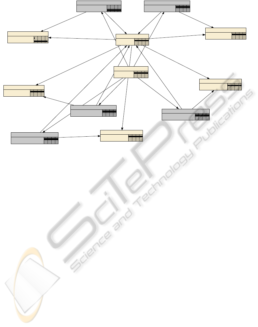
Figure 4: Bayesian Network Example.
tion and the cluster correlation disagree then the
reliability is set to 2% (reliable) and 98%
(unreliable).
4.1.4 Bayesian Network
In our Bayesian network, the existence of a tremor at
a particular cluster is depicted in the center of the
network labeled as ClusterYTremor, where ‘Y’
denotes the node number. Figure 4 shows an
example Bayesian Network for node 3. It should be
noted that in this phase we do not attempt to
determine whether a tremor has occurred. However,
the existence of a tremor is a factor that influences
the seismic sensor correlation and the cluster
correlations which ultimately determine the seismic
reliability of the data. Hence, ClusterYTremor lies at
the center of our network. It should be noted that we
did not need to input whether or not a tremor was
occurring into our Bayesian network as it was not
assumed that this was known. Instead it was
assumed that there was an equal probability of a
tremor occurring or not occurring. Once some
known data, specifically seismic data correlations,
were input into the Bayesian network, it would
automatically adjust the probability of a tremor
occurring. In addition to the ClusterYTremor nodes
in our Bayesian networks, there are other nodes:
NYSeismicSensorCorrelation, where Y is the sensor
N’s node number. Similar to the ClusterYTremor
nodes the value of the ClusterYCorrelation is not
definitively known. However, unlike the
ClusterYTremor node, the probability of the
ClusterYCorrelation is not 50/50. Because we had
additional knowledge about the cluster correlation
we could impart this knowledge into the Bayesian
network in the form a correlation table.
We imparted this knowledge into the table in the
form of probabilities. The final nodes in our
Bayesian networks are labelled
NYSeismicDataReliabiliy, where Y is the nodes
number (N2SeismicDataReliability). This was
represented by a percentage of the confidence that
we had in node Y’s seismic data and it was
computed and returned as the result of executing our
Bayesian network.
Once we determine the data reliability for all the
data streams, we use it as input into Phase II in order
to obtain an optimal data subset.
4.2 Phase II Knapsack Optimization
Phase II of our optimal data selection model uses the
data reliabilities assigned in Phase I and the
available bandwidth as input (refer Figure 5). In
OASIS, our resource constrained wireless sensor
network bandwidth was a limiting factor which had
to be conserved. As mentioned above, we had 16
sensor nodes, each of which were attached to
multiple, continuously sampling high fidelity
N2SeismicSensorCorrelation
High
Low
100
0
Cluster3Correlation
High
Low
98.0
2.00
Cluster3Tremor
Tru e
False
100
0 +
N1SeismicSenorCorrelation
High
Low
0
100
N10SeismicSensorCorrelation
High
Low
100
0
N1SeismicDataReliability
Reliable
Unreliable
3.96
96.0
N2SeismicDataReliability
Reliable
Unreliable
98.0
1.96
N10SeismicDataReliability
Reliable
Unreliable
98.0
1.96
N3SeismicDataReliability
Reliable
Unreliable
98.0
1.96
N17SeismicSensorCorrelation
High
Low
100
0
N17SeismicDataReliability
Reliable
Unreliable
98.0
1.96
N3SeismicSensorCorrelation
High
Low
100
0
PECCS 2011 - International Conference on Pervasive and Embedded Computing and Communication Systems
48

sensors. Each sensor node had a seismic, an
infrasonic, and a lightning sensor which were
sampled at a 100Hz, 100Hz, and 10Hz, respectively.
Due to the large amount of data being continuously
sampled and the limited bandwidth that was being
shared between the 16 nodes, it was not possible for
all of the data from all of the nodes to be transmitted
in real-time. The network bandwidth problem was
exasperated by the funnelling of data to a sink point
for transmission to an access point. Therefore, we
had to determine at any specific point in time which
was the “best” data to be sent. To decide what the
“best” data was, we needed to use the confidence
parameters determined by the Bayesian network and
optimize the bandwidth using a 0-1 Knapsack
approach, as shown in Figure 5, and discussed
thoroughly in the remainder of this section.
We used the confidence parameters because they
allowed us to reflect our belief in the correctness or
accuracy of the data in our decision. For example, if
some of the data had a confidence parameter of 15%
we would probably not have wanted to use our
valuable bandwidth to transmit such unreliable data.
The reason that we needed to optimize the
bandwidth and not just “fill up” all of the bandwidth
with the highest priority data was due to the
bandwidth sharing and funnelling effect of the
network topology of our sensor network. Further, we
need to minimize the bandwidth usage (by not
transmitting unreliable data) while maximizing the
return (high priority packets).
Figure 5: Knapsack Optimization.
In general, the knapsack optimization technique
originated from the class of problems using fixed
sized knapsack in which the user wants to carry the
most valuable items while minimizing the weight
that they had to bear. The 0-1 knapsack problem is
the most common type of knapsack problem in
which the number of each item is limited to either 0
or 1. Generally speaking, in a bounded knapsack
problem this number does not have to be limited to
one but may be any integer less than y, as specified
by the user. However, for our scenario each data
stream was unique, we never had duplicates of the
same data stream so it followed that we would use
the 0-1 knapsack approach.
Let us first define a value v
i
and a weight w
i
to be
associated with each of the data streams. Further, we
also had to assign a maximum weight, MW which
the entire network could not exceed. In our scenario,
the value, v
i
, of each item was the confidence
parameter. The weight, w
i
, associated with each data
stream was the cost of transmission in terms of
bandwidth. Finally, MW was the limiting bandwidth
available within the network. Our goal, which was to
minimize the weight w
i
while maximizing the value
received v
i
, is defined formally below in Equation 2
and Equation 3. Note, j
i
is the number of each of the
data streams which in our scenario was restricted to
0 or 1.
}1,0{∈∀j
(2)
Equation 2: Weight Maximizing.
}1,0{∈∀j
(3)
Note that for n items if we were to use a brute
force technique and compute all possible
combinations of the n data steams then this would
require 2
n
combinations to be computed. Thus, this
brute force approach has a computational
complexity, which is NP-complete. However, we
use a pseudo-polynomial time dynamic
programming solution, which reduces the
complexity to O(nW), which for known inputs is
weakly NP-complete and can be computed.
We input the confidence parameter and the
available bandwidth into the 0-1 knapsack
optimization algorithm. The output of this algorithm
is the optimum data subset. More specifically this is
a decision regarding the data, some subset i of our
total data set z, that would optimize our resources by
minimizing the cost while maximizing the return.
Thus, in choosing several items, say b items, we had
a choice, we could either add another item, say b+1,
or we could just have b items. If adding the
additional b+1 item would cause the total weight of
the subset, say w
sb
, to exceed the maximum weight
MW then item b+1 could not be added. However, if
∑
=
n
i
ii
jv
0
∑
=
≤
n
i
ii
MWjw
0
DATA RELIABILITY AND DATA SELECTION IN REAL TIME HIGH FIDELITY SENSOR NETWORKS
49

adding item b did not cause MW to be exceeded then
b+1 could be added. We chose to add item b+1 if
adding it would increase the confidence of the subset
(if v
sb+1
> v
sb
), otherwise (if v
sb+1
<= v
sb
) we
excluded it. It should be noted that the algorithm
only determines the maximum confidence that can
be achieved. It does not tell us which items attain
that confidence. In order to get the items we had to
additionally “mark” each item that should be
included. The items that should be included are the
ones that increase the overall confidence of the
subset (this is denoted v
sb+1
> v
sb
). The
implementation is discussed in detail in (Peterson,
2010).
5 EXPERIMENTS AND RESULTS
To provide input to Phase I, we emulated a
continuously changing stream of seismic data which
encompassed the different scenarios that we
expected to see on a volcano. We used 4 different
experimental setups. The first two experiments
consisted of real sensor data (with added tremor
points) while the second two experiments consisted
of random data with randomly occurring tremors and
random data with exponentially occurring tremors,
respectively. We divided each of the four
experiments into six time periods (for a total of 24
time periods), where each period represented a
specific scenario. It was important to use well
controlled data streams in which we knew which
sensors data streams contained bad or erroneous data
to be able to definitively state if the algorithms used
in the evaluations were accurately determining the
reliability.
In the experiments that will be described next,
we use the results from Phase I as input to Phase II
(as depicted in our model) and let the results for the
optimal data selection from both phases be
compared with other schemes, including schemes
that use various threshold values (expert knowledge)
or averaging for data selection.
We used the number of high priority nodes
selected (i.e., the number of high priority, high
reliable data selected) as the metric to measure the
accuracy of our algorithm. In general, our algorithm
selected more optimum nodes than the other
algorithms. We did this by selecting the nodes with
lower bandwidth requirements. Additionally our
algorithm also included additional nodes because we
continued to include nodes in the optimized subset
until we consumed all the remaining bandwidth.
In the previous section, we stated that we used
the individual data streams reliability parameters
from the Bayesian network. However, in our
discussion of the Knapsack implementation we said
that the value v
i
, of each data stream was the
confidence parameter. This confidence parameter is
a combination of both the reliability parameter and
the seismic data priority of each data stream both of
which are derived from Phase I. We choose to utilize
this in order to assign a seismic data priority to each
data flow. This allowed us to give more importance
to nodes in area(s) where we believed activity
(seismic tremor) was occurring. This was very
important as we were not just interested in the most
reliable data but rather the most significant reliable
data. Thus, we simply combined (through a
summation) the seismic data reliability and the
seismic data priority into one entity, the confidence
parameter, v
i
. We implemented our algorithm in
MATLAB.
5.1 Experiment Scenarios
In order to evaluate our algorithm, we compared it
with three other commonly used algorithms (Ahmen
et al., 2005) (Bettini et al., 2007). The first algorithm
(referred to as Threshold) used a threshold of 90% as
advised by the Earth Scientists. However, as
discussed in Phase I, a single low value will result in
an average below 90% for the entire cluster. Thus,
we also evaluated using a low threshold of 75% to
accommodate this (referred to as Low Threshold). In
addition we also tested it using the median of all
data values, excluding all values below the median
(referred to as Median). This is a simplified version
of our voting algorithm (from Phase I). We also
made the assumption that all of the algorithms start
selecting the nodes numerically beginning with the
lowest number (for consistency).
As previously stated, our first experiment
consisted of real seismic data “injected” with
seismic tremor points as well as faulty data. We
performed and collected the results for all four
experiments, each having six periods for a total of
96 different results. The trace scenarios for Periods I
– VI are as follows.
| Period I: Tremor detectable by all nodes
| Period II: Tremor detectable by all clusters
y Nodes 8 and 17 produce some erroneous data.
| Period III: Tremor detectable by all clusters
y Nodes 1, 6, 11, 16 some erroneous data
| Period IV: Tremor detectable by Clusters 3 & 4
y Nodes 1,2,3,10,17
y Nodes 4,5,6
| Period V: Tremor detectable by Clusters 3 and 4
PECCS 2011 - International Conference on Pervasive and Embedded Computing and Communication Systems
50

y Nodes 1, 2, 3, 10, 17 (4 good, 1 bad)
y Nodes 4, 5, 6 (all good nodes)
y Nodes 8, 17 some erroneous data
| Period VI: Tremor detectable by Clusters 3 and 4
y Nodes 1, 2, 3, 10, 17 (4 good, 1 bad)
y Nodes 4, 5, 6 (2 good, 1 bad)
y Clusters 1 and 2 cannot detect tremor and also
each have one node with some erroneous data.
y Nodes 1, 6, 11, 15 erroneous
5.2 Results
For all of the experiments we represented the 16
nodes with their id number in matrix M = [1, 2, 3, 4,
5, 6, 8, 9, 10, 11, 12, 13, 14, 15, 16, 17]. The weights
of the nodes correspond to the bandwidth that was
required to transmit the data from that node to the
sink node (in number of hops) and was given by
weights = [2, 2, 2, 1, 1, 1, 3, 3, 2, 3, 3, 3, 3, 3, 3, 2].
The SeismicDataReliabilty and the
SeismicDataPriority (both resulting from the
Bayesian network in Phase I) were each represented
in a matrix. In the interest of space we will not
display all of the SeismicDataReliabilty and the
SeismicDataPriority matrices. As an example the
matrices for Experiment I, Phase III are:
SeismicDataReliability = [3.96, 98, 98, 70.6, 70.6,
31.4, 90.2, 90.2, 98, 11.8, 90.2, 90.2, 90.2, 90.2,
11.8, 98]
SeismicDataPriority = [0, 100, 100, 100, 100, 0,
100, 100, 100, 0, 100, 100, 100, 100, 0, 100]. These
two matrices were added together to get the resulting
confidence parameter that is used as input into the
algorithms. Confidence parameter = [3.96, 198, 198,
170.6, 170.6, 31.4, 190.2, 190.2, 198, 11.8, 190.2,
190.2, 190.2, 190.2, 11.8, 198].
We used two measures to evaluate the algorithms:
accuracy (explained below) and the percentage of
the optimal data selected. It should be noted that in
our volcanic monitoring scenario all the data is not
treated equal. Rather, some of the data can be
categorized as good or error free data, while other
data is referred to as bad or erroneous data.
Additionally, the good data must further be
categorized as good data which is generated from a
node that is physically located in an area of activity,
and hence has a higher priority or good data that is
generated from a node that is in a non-active area
and has a lower priority. We must adhere to these
distinctions to correctly measure the accuracy of the
algorithms.
We designed a point system to measure the
accuracy of the algorithms such that it reflects the
information related to the type of data selected by
the algorithm. The accuracy of the algorithm is
initially set to 0. Each algorithm is then assigned
points based on the type of node it includes in the
optimal data subset. For each node in the optimal
subset that is erroneous we add “-1” to its current
accuracy. Each good node that is included in the
optimal subset “+1” or “+2” is added to the accuracy
for low priority and the high priority nodes,
respectively.
Figures 6 – 9 show the accuracy of all the
algorithms for time periods I – VI under different
network bandwidths. The available bandwidth refers
to the space available to transmit the data. Thus,
high bandwidth indicates that 83% of the data is
allowed to be transmitted, while medium high,
medium, and low can handle 53%, 26%, and 13% of
allowable data, respectively. In Period I of Figures 6
– 8, all four algorithms performed equally. This was
as expected as this time period contained no activity
and had no erroneous data; rather it was used as a
validity test. When the available bandwidth was low,
Figure 9, we performed better due to our
optimization of the nodes and their associated
bandwidth requirements. In all four figures you can
see that in relation to the other algorithms, ours
showed the most improvement in Periods III, V, and
VI. This is because those were the time period that
contained some erroneous data. Additionally, you
can see that the increase in the amount of accuracy
points that our algorithm gains versus the other
algorithms is inversely related to the available
bandwidth. Thus, while our algorithm never
performed worse than the competition, it displays
the most gains when the bandwidth resources are
restricted and erroneous data is present.
The second metric that we used to evaluate our
optimum data selection algorithm was a measure of
the percentage of the optimal data that was chosen.
By optimal data, we refer to all of the data that does
not contain errors. In order to compute the
percentage, as shown in Figures 10 – 13, we took the
ratio of the total number of good nodes that were
selected in the optimum data set to the total number
of nodes that were in the entire sample. From the
results it is evident that the percentage of increase is
directly proportional to the available bandwidth.
Thus, it is expected that when the bandwidth is
limited, the total number of nodes selected is also
reduced. However we can refer to the relative gain
between algorithms in order to compare their results.
As demonstrated in Figure 10, when the
bandwidth is limited, our algorithm outperformed
others in all cases. Again, it is demonstrated in all of
the figures that we showed the greatest improve-
DATA RELIABILITY AND DATA SELECTION IN REAL TIME HIGH FIDELITY SENSOR NETWORKS
51
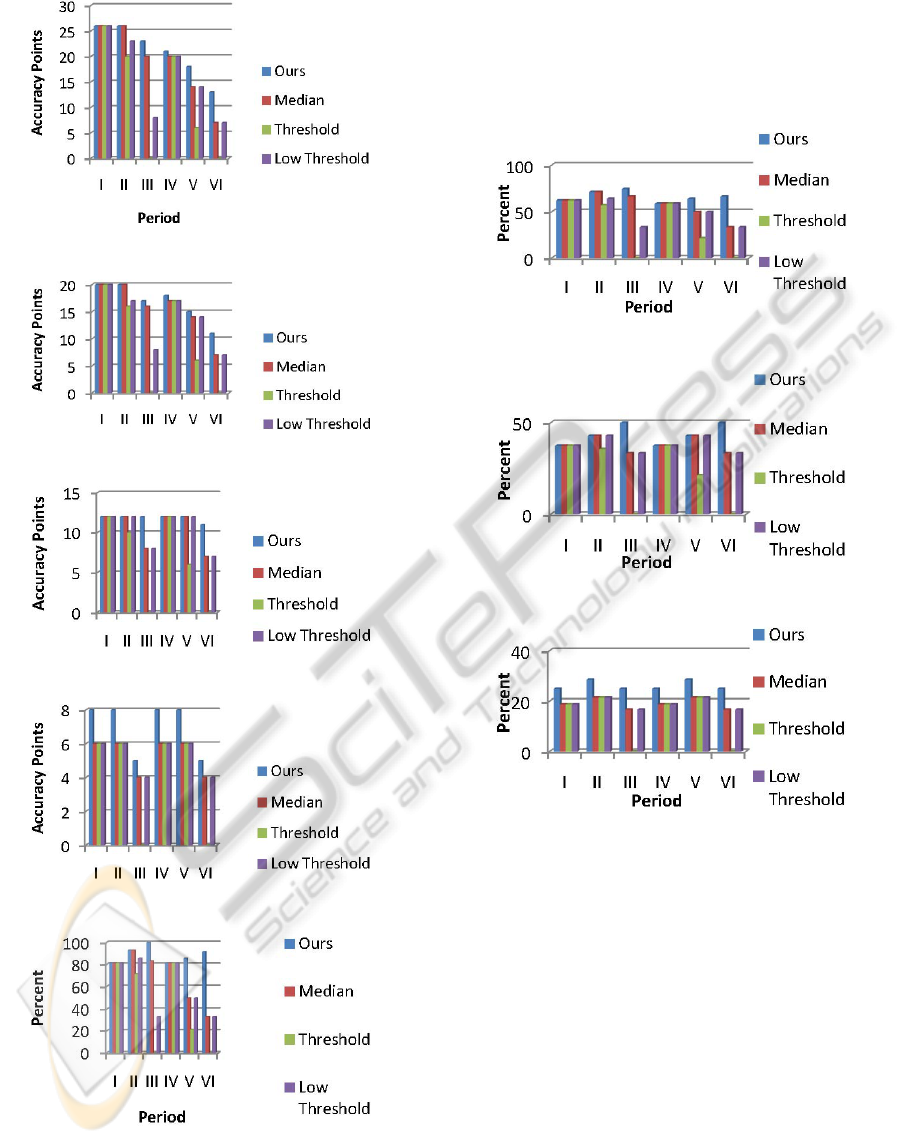
Figure 6: Accuracy for High Bandwidth.
Figure 7: Accuracy for Medium High Bandwidth.
Figure 8: Accuracy for Medium Bandwidth.
Figure 9: Accuracy for Low Bandwidth.
Figure 10: Good Data Selected High Bandwidth.
ments in the periods where there was erroneous data
present. This is particularly important because this
algorithm is not necessary if none of the data was
erroneous or if the bandwidth was such that all of
the data could be select. Rather it is when the
bandwidth is restricted and the data is not all good
that we require optimization of the subset selection
algorithm.
Figure 11: Good Data Selected Medium High Bandwidth.
Figure 12: Good Data Selected Medium Bandwidth.
Figure 13: Good Data Selected Low Bandwidth.
6 CONCLUSIONS
AND FUTURE WORK
Optimal data selection has become an important
issue in environment monitoring, where high-
fidelity, continuous data samples are used. We
designed, implemented, and tested our optimal data
selection model system for wireless sensor networks.
Our model is composed of two phases: one to
identify the confidence in the data and second to
optimize the selection of the data based on its
reliability and availability of network bandwidth.
Our analysis showed that when compared to other
algorithms, our optimal data selection model was
able to significantly outperform existing algorithms.
PECCS 2011 - International Conference on Pervasive and Embedded Computing and Communication Systems
52

While we implemented and tested our algorithm
in a volcanic monitoring scenario, our work is not
constrained to this arena. The proposed optimal data
selection model is ideally suited to many resource
constrained wireless sensor networks where data
quality and data selection are important. Further, we
are extending this optimal data selection model into
a larger context modeling framework that also
determines when a tremor occurs, as opposed to
other events such as a rock falling, and its location.
REFERENCES
Ahmen, B., Lee, Y-K., Lee, S., Zhung, Y., 2005. ‘Scenario
Based Fault Detection in Context-Aware Ubiquitous
Systems using Bayesian Networks’, Computational
Intelligence for Modelling , Control and Automation,
pp. 414-420.
Bettini, C., Brdiczka, O., Henricksen, K., Indulska, J.,
Nicklas, D., Ranganathan, A., Riboni, D., 2009. ‘A
survey of context modelling and reasoning
techniques’Pervasive and Mobile Computing, pp. 161-
180.
Bettini, C., Maggiorini, D., Riboni, D., 2007. ‘Distributed
Context Monitoring for the Adaptation of Continuous
Services’, World Wide Web, Springer Netherlands.
Kumar, et al., 2003. ‘PICO: A Middleware Framework for
Pervasive Computing’, IEEE Pervasive Computing,
pp. 72-79.
Survey, U.S. Geological. www.usgs.gov/
Lee, D., Meier, R., 2007. ‘Primary-Context Model and
Ontology: A Combined Approach for Pervasive
Transportation Services’, IEEE Pervasive Computing
and Communications Workshops, pp. 419-424.
Peterson, N., 2010. ‘Adaptive Context Modeling and
Situation Awareness for Wireless Sensor Networks’,
Ph.D. dissertation, Dept. Elect. Eng. and Competer
Science, Washington State Univ., Pullman, WA.
Peterson N., et al., 2008. ‘Tiny-OS Based Quality of
Service Management in Wireless Sensor Networks’,
Hawaii International Conference on System Sciences,
pp. 1-10.
Song, W., et al., 2008. ‘Optimized Autonomous Space In-
situ Sensor-Web for Volcano Monitoring’, IEEE
Journal of Selected Topics in Earth Observations and
Remote Sensing, pp. 1-10.
DATA RELIABILITY AND DATA SELECTION IN REAL TIME HIGH FIDELITY SENSOR NETWORKS
53
