
THE SPIRAL FACETS
A Unified Framework for the Analysis and Description of 3D Facial Mesh Surfaces
Naoufel Werghi, Harish Bhaskar
Dept. of Computer Engineering, Khalifa University, Sharjah Campus, Sharjah, U.A.E.
Youssef Meguebli, Haykel Boukadida
School of Science and Techniques, University of Tunis, Tunis, Tunisia
Keywords:
3D Face descriptors, Spiral facets, Feature localization, Geodesic curves, 3D Face orientation.
Abstract:
In this paper, we describe a framework for encoding 3D facial triangular mesh surface. We derive shape
information from the triangular mesh surface by exploiting specific arrangements of facets in the model. We
describe the foundations of the framework and adapt the framework for several original applications including:
face landmark detection, frontal face extraction, face orientation and facial surface representation. We validate
the framework through experimentation with raw 3D face mesh surfaces and demonstrate that the model allows
simpler implementation, more compact representation and encompasses rich shape information that can be
usefully deployed both locally and globally across the face in comparison to other standard representations.
1 INTRODUCTION
Face recognition is a central problem in biomet-
ric authentication, with applications including visual
surveillance and security. However, 2D face recogni-
tion systems are complicated by sensitivity to illumi-
nation conditions and pose variation. A popular al-
ternative to such 2D image-based systems is the use
of 3D face images whose richness and completeness
is often exploited to contribute in solving the inher-
ent limitations of 2D systems. However, there is a
growing need to faithfully encode raw 3D facial mesh
surface into a simple, structured and compact facial
representation.
There exist competing approaches to model 3D fa-
cial mesh surfaces. 3D shape can be represented in-
dependent of the co-ordinate system using the object-
centric representations. Such representations have in-
vited much attention in recent years due to their in-
variance to geometric transformations and their po-
tential to produce an reliable metric for facial shape
comparison.
In this paper, we propose a topological framework
for encoding 3D facial mesh surface that is concise
(encompasses dimensionality reduction, as a means
of improving the efficiency, or allowing the data com-
pression) and computationally efficient. We denote
this representation as the ”spiral facets” and show
how this representation can be neatly adapted to ad-
dress several applications including but not restricted
to: facial landmarks detection, frontal face extraction,
face shape description and face pose computation.
2 RELATED WORK
In the context of 3D face recognition, we can catego-
rize the face shape representations into three classes,
namely: Local features representation, global feature
representation and hybrid representations.
Local feature representation methods employ fea-
tures derived from local face surface (at a limited
neighborhood). These attributes typically include cur-
vature measures (Moreno et al.,2006), and point sig-
natures (Chua et al.,2000). The derivation of local
features is performed with differential geometry tech-
niques that are intrinsically vulnerable to scaling and
data deficiencies (e.g., non-uniform resolution, pres-
ence of noise).
In contrast to the local representation, in global
representation, the facial features are derived from
the whole 3D face data. Wu (Wu et al.,2003) used
vertical and horizontal profiles of faces and Xu (Xu
et al.,2008) derived invariant curve and surface mo-
ments from 3D face data. In these methods, match-
30
Werghi N., Bhaskar H., Meguebli Y. and Boukadida H..
THE SPIRAL FACETS - A Unified Framework for the Analysis and Description of 3D Facial Mesh Surfaces.
DOI: 10.5220/0003362300300039
In Proceedings of the International Conference on Computer Vision Theory and Applications (VISAPP-2011), pages 30-39
ISBN: 978-989-8425-47-8
Copyright
c
2011 SCITEPRESS (Science and Technology Publications, Lda.)

ing is performed by evaluating the similarity between
these entities. Other methods (Irfanoglu et al.,2004;
Lu and Jain,2005) superimpose the whole query 3D
facial image with the stored instances in the database,
and then evaluate the degree of overlapping to decide
whether or not they match. These approaches are
limited by their high computational cost. In (Lee et
al.,2003; Xu et al.,2004b) authors, extend the eigen-
faces paradigm developed in 2D face recognition to
the 3D case. This paradigm operates on a range or
depth image in which the pixel intensity represents
the ’z’ coordinate. However, these methods have in-
herited some of the shortcomings of 2D face identifi-
cation, particularly with regard to the face pose, self-
occlusion and scaling. Other representations have
been developed based on geodesic entities (Bronstein
et al.,2003; Berretti et al.,2006; Samir et al., 2009),
these approaches aimed also to address face shape de-
formation. So did (Kakadiaris, 2007) with their de-
formable face model.
Finally, hybrid representation combines local and
global facial features. These methods were moti-
vated by psychological findings asserting that humans
equally rely on both local and global visual informa-
tion. Pan (Pan et al.,2003) augmented the eigenface
paradigm with face profile. Xu (Xu et al.,2004a) de-
veloped a face representation defined by a measure
of the similarity between the 3D face image and a
3D face template, and local shape variation around
local facial. landmarks (e.g., eyes and nose). Al-
Osaimi (Mian et al.,2007) employed a 2D histogram
that encompasses rank-0 tensor fields extracted at lo-
cal points of the facial surface and from the whole
face depth map data.
3 CONTRIBUTIONS
& STRUCTURE
The framework described in this paper, extracts or-
dered structured patterns from 3D triangular mesh
surface for a simple representation of facial surfaces.
We acknowledge that there are a number of repre-
sentations of 3D facial surfaces in the literature and
therefore, we list a set of 4 main characteristics of our
proposed ”spiral facets” representation that will dis-
tinguish it from other close face shape representation
(Berretti et al., 2006; Samir et al., 2009). These char-
acteristics include: a) simplicity and compactness:
the spiral facet representation is a single data struc-
ture, b) generalization: the facet spiral is a general-
ized representation of other popular 3D facial surface
representations and it is possible that we can derive
for example, the approximate geodesic rings structure
from the spiral facet, c) processing efficiency: our
representation also does not require any form of mesh
pre-processing, whereas in most other method mesh
regularization is often required and finally, d) compu-
tational complexity: out method is computationally
more efficient. As we will explained in the end of
Section 4, we infer a complexity of (O(n)) in com-
parison to O(nlog(n)) in (Berretti et al., 2006; Samir
et al., 2009) which also requires a mesh regularization
of complexity O(n).
The other main novelty of the proposed frame-
work is in the adaptability of the framework for sev-
eral original applications including: a) nose tip local-
ization, b) frontal face extraction, c) 3D face shape
modeling d) 3D face pose computation and e) nose
profile identification.
We begin by describing our framework of 3D fa-
cial surface representation in Section 4. We then elab-
orate different applications of the proposed frame-
work in section 5 and conduct systematic experiments
on varied datasets for nose tip localization 5.1, 3D
frontal face extraction 5.2, face shape description 5.3,
3D face pose computation 5.4 and nose profile iden-
tification 5.5. In Section 6 we present concluding re-
marks and directions of future work.
4 THE SPIRAL FACETS
FRAMEWORK
In our framework, we derive a 3D facial surface rep-
resentation by constructing novel structured and or-
dered patterns in a 3D face triangular mesh surface.
The triangular mesh surface representation though is
simple, lacks an intrinsic ordered structure that allows
the facets in the mesh to be browsed systematically.
Consequently, storing the facets in the facet array is
usually arbitrary and does not follow any particular
arrangement. Therefore processing and analyzing tri-
angular mesh surfaces are more complex compared
with other intrinsically ordered shape modalities such
as range images. According to our framework, we
construct patterns exploiting topological properties of
a triangular mesh surface. These patterns include con-
centric rings of facets that can also be arranged in a
spiral-wise fashion. Our framework has been inspired
from the observation of the arrangement of triangu-
lar facets lying on closed contour of edges (Figure
1.a). From this, we can categorize the facets into two
groups: 1) facets having an edge on that contour that
seem to point outside the area delimited by the con-
tour (e.g. fout
1
and f out
2
in Figure 1.a). And 2)
facets having a vertex on the contour that point inside
the contour’s area. The facets in the second group
THE SPIRAL FACETS - A Unified Framework for the Analysis and Description of 3D Facial Mesh Surfaces
31
have an effect of filling gaps between facets in the
first group. We call these two groups of facets as Fout
and Fgap facets and together, they form a kind of ring
structure. Using this ring facets we can derive a new
group of Fout facets that are one-to-one adjacent with
the Fgap facets of the previous ring, that will in-turn
form the basis of the subsequent rings (Figure 1.b).
We iterate this process to obtain a group of concen-
tric rings. When the initial contour is composed of
the edges of a given triangular facet, the rings will be
centered at that particular facet (Figure 1.c). More-
over, by imposing the last facet in the current ring to
be connected to the first facet in the subsequent ring,
we obtain a sequence of facets arranged on a spiral-
wise fashion, i.e. sequence of facets starting at the
root facet and following a spiral path on the facial sur-
face. We dubbed this arrangement ”the spiral facet”.
(Figure 1.d). We also note that from the root triangle
3 different spiral facets can be generated depending
on the chosen facet among the three facets adjacent to
the root facet.
The algorithm for constructing a facet spiral start-
ing at a given facet t is as follows:
Algorithm GetSpiralFacets.
Rings = [t] , FoutFacets ← facets adjacent to t
For i=1: Number of rings
GapFacets ← FillGap(FoutFacets)
Ring ← FoutFacets + GapFacets
Append Ring to Rings
NewFoutFacets ← GetFoutFacest
(GapFacets,FoutFacets)
FoutFacets ← NewFoutFacets
End For
The algorithm GetSpiralFacets has computational
complexity of O(n) where n is the number of facets
in the facet spiral.
One of the main interesting characteristics of the
spiral facets representation is that facets at a given
ring are approximately at the same geodesic distance
from the root facet. The geodesic distance can be ap-
proximated to RingNumber ×L, where RingNumber
is the ring’s number in the facet spiral, and L is the
average length of the triangle’s edge. Therefore, it is
possible to use the spiral facets as a low cost alterna-
tive for computing an approximation of iso-geodesic
contours on the facial surface, compared to the stan-
dard O(nlog(n)) Dijkstra algorithm (Cormen et al.,
2001) (employed in (Samir et al., 2009)) and the
O(nlog(n)) fast marching method (Sethian and Kim-
mel, 1998) (used in (Berretti et al., 2006)). We com-
pute the geodesic path using the spiral facets in two
distinctive stages (Figure 1.e) . In the first step, the
spiral facets are expanded from a source facet until
inspired from the observation of the arrangement of
triangular facets lying on closed contour of edges
(Figure 1.a) . From this, we can categorize the facets
into two groups: 1) facets having an edge on that
contour that seem to point outside the area delimited
by the contour (e.g. fout
1
and f out
2
in Figure 1.a).
And 2) facets having a vertex on the contour that
point inside the contour’s area. The facets in the
second group have an effect of filling gaps between
facets in the first group. We call these two groups
of facets as Fout and Fgap facets and together, they
form a kind of ring structure. Using this ring facets
we can derive a new group of Fout facets that are
one-to-one adjacent with the Fgap facets of the
previous ring, that will in-turn form the basis of the
subsequent rings (Figure 1.b). We iterate this process
to obtain a group of concentric rings. When the initial
contour is composed of the edges of a given triangular
facet, the rings will be centered at that particular facet
(Figure 1.c). Moreover, by imposing the last facet in
the current ring to be connected to the first facet in
the subsequent ring, we obtain a sequence of facets
arranged on a spiral-wise fashion, i.e. sequence
of facets starting at the root facet and following a
spiral path on the facial surface. We dubbed this
arrangement ”the spiral facet”. (Figure 1.d). We
also note that from the root triangle 3 different spiral
facets can be generated depending on the chosen
facet among the three facets adjacent to the root facet.
The algorithm for constructing a facet spiral
starting at a given facet t is as follows:
Algorithm GetSpiralFacets
Rings = [t] , FoutFacets ← facets adjacent to t
For i=1: Number of rings
GapFacets ← FillGap(FoutFacets)
Ring ← FoutFacets + GapFacets
Append Ring to Rings
NewFoutFacets ← GetFout-
Facest(GapFacets,FoutFacets)
FoutFacets ← NewFoutFacets
End For
The algorithm GetSpiralFacets has computa-
tional complexity of O(n) where n is the number of
facets in the facet spiral.
One of the main interesting characteristics of
the spiral facets representation is that facets at a
given ring are approximately at the same geodesic
distance from the root facet. The geodesic distance
can be approximated to RingNumber × L, where
RingNumber is the ring’s number in the facet spiral,
and L is the average length of the triangle’s edge.
3
fout
fout
fout
1
2
7
fg
fg
1
2
v
v
v
v
v
v
1
2
3
4
5
v
6
7
vout
vout
vout
1
2
7
fout
fout
fout
1
2
7
fg
fg
1
2
v
v
v
v
v
v
1
2
3
4
5
v
6
(a) (b)
(c) (d)
(e)
(f)
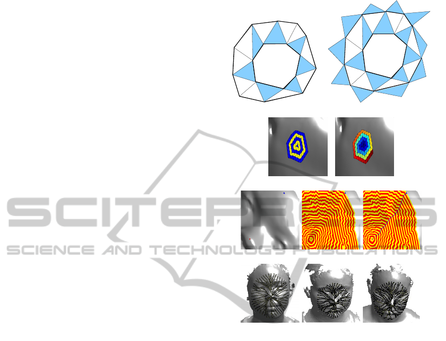
Figure 1: a:Fout facets (dark) on the contour E
7
:
(v
1
,v
2
,..v
7
). The Fgap facets (clear) bridge the gap be-
tween pairs of consecutive Fout facets. b :Extraction of the
new Fout facets. Notice that the new Fout facets are one-
to-one adjacent to the Fgap facets. c: An examples of facet
spiral and its concentring rings. d: The same facet spiral
where the facets are arranged spiral-wise. e: Example of
a geodesic path computation: The facet spiral is expanded
from a source facet on the nose tip until the the destina-
tion facet is reached, then the geodesic path is extracted by
tracing back the source facet. f: examples of geodesic paths
between the nose tip and facets on a periphery ring of a facet
spiral.
Therefore, it is possible to use the spiral facets as a
low cost alternative for computing an approximation
of iso-geodesic contours on the facial surface, com-
pared to the standard O(nlog(n)) Dijkstra algorithm
(Cormen et al., 2001) (employed in (Samir et al.,
2009)) and the O(nlog(n)) fast marching method
(Sethian and Kimmel., 1998) (used in (Berretti et al.,
2006)). We compute the geodesic path using the
spiral facets in two distinctive stages (Figure 1.e) . In
the first step, the spiral facets are expanded from a
source facet until the destination facet is reached (i.e.,
found in the last ring). In the second step, the rings
(f)
Figure 1: a): Fout facets (dark) on the contour E
7
:
(v
1
,v
2
,..v
7
). The Fgap facets (clear) bridge the gap be-
tween pairs of consecutive Fout facets. b :Extraction of the
new Fout facets. Notice that the new Fout facets are one-
to-one adjacent to the Fgap facets. c: An examples of facet
spiral and its concentring rings. d: The same facet spiral
where the facets are arranged spiral-wise. e: Example of
a geodesic path computation: The facet spiral is expanded
from a source facet on the nose tip until the the destina-
tion facet is reached, then the geodesic path is extracted by
tracing back the source facet. f: examples of geodesic paths
between the nose tip and facets on a periphery ring of a facet
spiral.
the destination facet is reached (i.e., found in the last
ring). In the second step, the rings are browsed back-
wards, starting from the destination facet, and reiter-
ated looking for the nearest connected facet in the pre-
vious ring until the source facet is reached. Since the
algorithm GetSpiralFacet intrinsically computes the
connectivity between facets in adjacent rings, the sec-
ond stage has a complexity of O(RingNumber). (Fig-
ure 1.f) depicts facets on the geodesic paths between
the nose tip and facets located at a given ring of the
facet spiral.
VISAPP 2011 - International Conference on Computer Vision Theory and Applications
32

5 APPLICATIONS
In this section of the paper, we exhibit the generality
of the spiral facets framework by adapting it for sev-
eral 3D face applications. One of the critical steps to-
wards face recognition is the localization of features.
In the initial attempt to localize 3D facial features us-
ing the ”spiral facets” representation, we first present
the nose tip detection application in Section 5.1. We
substantially elaborate on this part since the rest of
the applications depends on it. Next, we describe the
algorithm to extract the frontal face from the raw 3D
face scan by propagating rings starting from the de-
tected nose tip in Section 5.2. Face shape descrip-
tion and pose identification are also important com-
ponents particularly to model based matching of 3D
faces. In Sections 5.3,5.4 we explore an approach
for face shape description and face pose computation
using the spiral facets framework. Finally, we also
exploit the geodesic properties of the spiral facets to
extract the nose profile from 3D face scans in Sec-
tion 5.5.
5.1 Nose Tip Detection
Face landmarks detection is critical to face recogni-
tion and nose tip detection in particular has a capital
role due to its center position and saliency. A majority
of 3D face analysis techniques are anchored to detect-
ing the nose tip. The problem of nose tip detection has
been approached using heuristic rules-based methods
(Colbry et al., 2005; Heseltine et al., 2008). Such
methods requires a restricted face pose. This issue
was addressed to some extent by shape descriptors-
based methods (Segundo et al., 2007; Wang et al.,
2008) that are specifically invariance to geometric
transformation. However, the presence of noise has
often affected the reliability of such systems. Statisti-
cal methods (Ruiz and Illingworth,2008; Romero and
Pears, 2009) employed a landmarks model, obtained
via training. This model is registered to the face data
in order to get an approximate landmark locations,
which are further refined in an iterative manner. This
method inherits the problems of model registration;
such as the need of prior pose information. Apart
of (Xu et al., 2006) most approaches that dealt with
face landmarks detection treated a pre-processed data,
in which the 3D face surface has been cropped and
smoothed. The method in (Xu et al., 2006) uses a hi-
erarchical filtering scheme employing shape descrip-
tors and a local nose tip shape model. The method
is robust, but, revealed cases of false detection for
some instance where clothing deformation matches
the nose tip statistical model.
We propose an application of the 3D spiral facets
for nose tip detection from raw 3D triangular mesh fa-
cial surfaces. Our method is inspired from the obser-
vation that the regions around some facial landmarks
are characterized by low mesh quality. These result
from gaps (in the nostrils) and reflection effects (at
the eyes) (see Figure 2.a). To measure and assess the
quality of the mesh surface, we present an original
framework using which we extract a group of candi-
date triangular facets. In the second stage of our algo-
rithm, we find the single facet that corresponds to the
nose tip from the group of candidate triangle facets
using a series of filtering steps.
5.1.1 Assessing the Regularity of the Mesh
Tessellation
The term mesh quality is context driven and tightly
linked to the subsequent use of the constructed mesh
(Frey and Borouchaki, 1999), therefore there is no
standard framework for assessing the quality of tri-
angular mesh surface for raw 3D facial surface scan.
are browsed backwards, starting from the destination
facet, and reiterated looking for the nearest connected
facet in the previous ring until the source facet is
reached. Since the algorithm GetSpiralFacet intrin-
sically computes the connectivity between facets in
adjacent rings, the second stage has a complexity
of O(RingNumber). (Figure 1.f) depicts facets on
the geodesic paths between the nose tip and facets
located at a given ring of the facet spiral.
5 Applications
In this section of the paper, we exhibit the gen-
erality of the spiral facets framework by adapting it
for several 3D face applications. One of the critical
steps towards face recognition is the localization of
features. In the initial attempt to localize 3D facial
features using the ”spiral facets” representation, we
first present the nose tip detection application in Sec-
tion 5.1. We substantially elaborate on this part since
the rest of the applications depends on it. Next, we
describe the algorithm to extract the frontal face from
the raw 3D face scan by propagating rings starting
from the detected nose tip in Section 5.2. Face shape
description and pose identification are also important
components particularly to model based matching of
3D faces. In Sections 5.3,5.4 we explore an approach
for face shape description and face pose computation
using the spiral facets framework. Finally, we also
exploit the geodesic properties of the spiral facets to
extract the nose profile from 3D face scans in Sec-
tion 5.5.
5.1 Nose Tip Detection
Face landmarks detection is critical to face recog-
nition and nose tip detection in particular has a
capital role due to its center position and saliency. A
majority of 3D face analysis techniques are anchored
to detecting the nose tip. The problem of nose tip
detection has been approached using heuristic rules-
based methods (Colbry et al., 2005; Heseltine et al.,
2008). Such methods requires a restricted face pose.
This issue was addressed to some extent by shape
descriptors-based methods(Segundo et al., 2007;
Wang et al., 2008) that are specifically invariance
to geometric transformation. However, the presence
of noise has often affected the reliability of such
systems. Statistical methods (Ruiz and Illingworth,
2008; Romero and Pears, 2009) employed a land-
marks model, obtained via training. This model
is registered to the face data in order to get an
approximate landmark locations, which are further
refined in an iterative manner. This method inherits
the problems of model registration; such as the need
of prior pose information. Apart of (Xu et al., 2006)
most approaches that dealt with face landmarks
detection treated a pre-processed data, in which the
3D face surface has been cropped and smoothed.
The method in (Xu et al., 2006) uses a hierarchical
filtering scheme employing shape descriptors and a
local nose tip shape model. The method is robust, but,
revealed cases of false detection for some instance
where clothing deformation matches the nose tip
statistical model.
We propose an application of the 3D spiral facets
for nose tip detection from raw 3D triangular mesh
facial surfaces. Our method is inspired from the
observation that the regions around some facial
landmarks are characterized by low mesh quality.
These result from gaps (in the nostrils) and reflection
effects (at the eyes) (see Figure 2.a). To measure and
assess the quality of the mesh surface, we present an
original framework using which we extract a group of
candidate triangular facets. In the second stage of our
algorithm, we find the single facet that corresponds
to the nose tip from the group of candidate triangle
facets using a series of filtering steps.
5.1.1 Assessing the regularity of the mesh
tessellation
The term mesh quality is context driven and tightly
linked to the subsequent use of the constructed mesh
(Frey and Borouchaki, 1999), therefore there is no
standard framework for assessing the quality of tri-
angular mesh surface for raw 3D facial surface scan.
Our proposed technique measures to what extent a tri-
(a) (b)
Figure 2: a: A sample triangular mesh facial surface. Notice
the mesh irregularities at the nostrils, and the the eyes areas.
b: Computation of the error ∆
3
at each facet. Dark areas
correspond to a large error.
angular mesh is close to an ideal mesh composed of
equal-sized equilateral triangles at a given neighbor-
hood. In such mesh, we can show easily that the num-
ber of triangles across the concentric rings that from
the facet spiral follow arithmetic progression:
(a) (b)
Figure 2: a): A sample triangular mesh facial surface. No-
tice the mesh irregularities at the nostrils, and the the eyes
areas. b): Computation of the error ∆
3
at each facet. Dark
areas correspond to a large error.
Our proposed technique measures to what extent
a triangular mesh is close to an ideal mesh composed
of equal-sized equilateral triangles at a given neigh-
borhood. In such mesh, we can show easily that the
number of triangles across the concentric rings that
from the facet spiral follow arithmetic progression:
nrt(n + 1) = nrt(n) + 12 (1)
where nrt(n) and nrt(n + 1) are the number of trian-
gles in the ring n and n + 1 respectively. Therefore,
the sequence
ˆ
η
n
in an ideal mesh, starting at a root
facet, is [12,24,36, ,12n]. This condition will not be
satisfied at surface areas where the uniformity of the
mesh tessellation is corrupted. Based on this, we pro-
pose the following local criterion for evaluating the
mesh tessellation uniformity.
∆
n
=
kη
n
−
ˆ
η
n
k
k
ˆ
η
n
k
, (2)
THE SPIRAL FACETS - A Unified Framework for the Analysis and Description of 3D Facial Mesh Surfaces
33

where η
n
(respectively
ˆ
η
n
) is the sequence represent-
ing the number of triangles across a group of n con-
centric rings in a arbitrary mesh (respectively an ideal
mesh). Figure 2.b depicts ∆
3
computed at each facet
of a sample 3D raw facial data.
5.1.2 Cascading filters
After computing the error ∆
n
(Figure 3.b), we retain
those facets having a ∆
n
above a certain threshold.
The group of facets extracted from this level of fil-
tering (dubbed Group1), contains a majority of facets
in the neighborhood of the nostrils and eyes and also
other facets spread mostly across the ears, clothes and
the periphery areas in the raw mesh surface (as in Fig-
ure 3.c). In the second level of our cascaded filter-
ing implementation, we apply prior information de-
rived from the topological characteristics of the raw
face scan to extract the central facets corresponding
to a potential landmark. As Figure 3.a shows, the
face scan is composed of several fragmented mani-
fold pieces which includes the face, parts of the hair,
neck, and upper torso. We initialize a two-phase filter
where in the first phase, facets from Group1 generat-
ing more than 18 rings are selected. By doing this,
we capture facets located within the vicinity of the
central face, and naturally discard those which are lo-
cated at the surface periphery or at small surface frag-
ments. We set the threshold to 18 as it is about half the
maximum number of rings in a typical facial surface.
In the subsequent phase, we select from the obtained
facets those scoring the 10 highest number of rings
(Figure 3.d). To these facets we add those locates at
their neighborhoods (by expanding 4 rings-facet spi-
ral around each one of them). We called the so ob-
tained group of facets, Group 2 facets.
In the third level, we employ a model-based
matching method based on the standard Geometric
Histogram (GH) local shape descriptor (Ashbrook et
al., 1998). The GH is a 2D accumulator that describes
a pairwise relationship between a central facet and
each of it surrounding facets within a given neighbor-
hood. This relationship in the form of the angles (α)
between the central facet normals and all the other
facets’ normals, and the range of perpendicular alge-
braic distances (ρ) from the plane in which the cen-
tral facet lies to all the other facets in the neighbor-
hood. These measurements are entered in the dis-
crete angle distance 2D accumulator, thus obtaining
a kind of distribution that characterizes the relation-
ship between the root facet and its neighbors. The
neighborhood is constructed by generating a six-rings
spiral facets around a central facet. At this level, the
GH of each candidate facet is matched with the sta-
tistical model of GH of the nose tip neighborhood.
nrt(n + 1) = nrt(n) + 12 (1)
where nrt(n) and nrt(n + 1) are the number of trian-
gles in the ring n and n + 1 respectively. Therefore,
the sequence
ˆ
η
n
in an ideal mesh, starting at a root
facet, is [12,24,36, ,12n]. This condition will not be
satisfied at surface areas where the uniformity of the
mesh tessellation is corrupted. Based on this, we pro-
pose the following local criterion for evaluating the
mesh tessellation uniformity.
∆
n
=
∥η
n
−
ˆ
η
n
∥
∥
ˆ
η
n
∥
, (2)
where η
n
(respectively
ˆ
η
n
) is the sequence represent-
ing the number of triangles across a group of n con-
centric rings in a arbitrary mesh (respectively an ideal
mesh). Figure 2.b depicts ∆
3
computed at each facet
of a sample 3D raw facial data.
5.1.2 Cascading filters
After computing the error ∆
n
(Figure 3.b), we retain
those facets having a ∆
n
above a certain threshold.
The group of facets extracted from this level of filter-
ing (dubbed Group1), contains a majority of facets
in the neighborhood of the nostrils and eyes and also
other facets spread mostly across the ears, clothes
and the periphery areas in the raw mesh surface (as
in Figure 3.c). In the second level of our cascaded
filtering implementation, we apply prior information
derived from the topological characteristics of the raw
face scan to extract the central facets corresponding
to a potential landmark. As Figure 3.a shows, the face
scan is composed of several fragmented manifold
pieces which includes the face, parts of the hair,
neck, and upper torso. We initialize a two-phase
filter where in the first phase, facets from Group1
generating more than 18 rings are selected. By doing
this, we capture facets located within the vicinity of
the central face, and naturally discard those which are
located at the surface periphery or at small surface
fragments. We set the threshold to 18 as it is about
half the maximum number of rings in a typical facial
surface. In the subsequent phase, we select from
the obtained facets those scoring the 10 highest
number of rings (Figure 3.d). To these facets we add
those locates at their neighborhoods (by expanding
4 rings-facet spiral around each one of them). We
called the so obtained group of facets, Group 2 facets.
In the third level, we employ a model-based
matching method based on the standard Geometric
Histogram (GH) local shape descriptor (Ashbrook
et al., 1998). The GH is a 2D accumulator that
(a) (b) (c)
(d) (e) (f)
(g)
Figure 3: Nose tip detection stages a: raw 3D face mesh
surface. b: computation of the mesh quality criterion ∆
n
. c:
Selection of the facets scoring a ∆
n
above a certain thresh-
old. d: Elimination of the facets at the periphery areas and
selection of the most central facets. e: Detection of candi-
date facets via Geometric Histogram matching. f: selection
of the nose tip facet. g: Detected nose tips on some face
samples.
describes a pairwise relationship between a central
facet and each of it surrounding facets within a
given neighborhood. This relationship in the form
of the angles (α) between the central facet normals
and all the other facets’ normals, and the range of
perpendicular algebraic distances (ρ) from the plane
in which the central facet lies to all the other facets in
the neighborhood. These measurements are entered
in the discrete angle distance 2D accumulator, thus
obtaining a kind of distribution that characterizes the
relationship between the root facet and its neighbors.
The neighborhood is constructed by generating a six-
rings spiral facets around a central facet. At this level,
the GH of each candidate facet is matched with the
statistical model of GH of the nose tip neighborhood.
This model is obtained from 100 face data samples,
whereby we averaged the 100 GHs derived from their
corresponding nose tip neighborhoods. The matching
criterion used to evaluate the closeness of two GHs h
i
and h
j
is the Bhattacharya distance:
D
i j
Bhattacharya
=
∑
α,ρ
h
i
(α,ρ)
h
j
(α,ρ). (3)
Since the nose tip can be located as an area rather
a single point, and the matching is performed using an
average model, we select the facets having a matching
(g)
Figure 3: Nose tip detection stages a: raw 3D face mesh
surface. b: computation of the mesh quality criterion ∆
n
. c:
Selection of the facets scoring a ∆
n
above a certain thresh-
old. d: Elimination of the facets at the periphery areas and
selection of the most central facets. e: Detection of candi-
date facets via Geometric Histogram matching. f: selection
of the nose tip facet. g: Detected nose tips on some face
samples.
This model is obtained from 100 face data samples,
whereby we averaged the 100 GHs derived from their
corresponding nose tip neighborhoods.
The matching criterion used to evaluate the close-
ness of two GHs h
i
and h
j
is the Bhattacharya dis-
tance:
D
i j
Bhattacharya
=
∑
α,ρ
p
h
i
(α,ρ)
q
h
j
(α,ρ). (3)
Since the nose tip can be located as an area rather
a single point, and the matching is performed using an
average model, we select the facets having a matching
score at a given distance from the maximum. This set
of facets, called Group 3, is defined by:
N = {t \Max
D
−5σ ≤ D
Bhattacharyya
(GH
t
,GH) ≤ Max
D
}
(4)
where sigma is the variance of Bhattacharyya dis-
tances between the GHs samples used for computing
the mean GH model. Figure 3.e depicts and instance
of this set. In the final level of our cascaded filtering
implementation, we further refine the location of the
nose tip by computing for each facet in Group 3, the
rank-2 tensor field (Mian et al., 2007)
T =
n
∑
i=1
a
i
~r
i
~r
i
T
A|~r
i
k
2
(5)
VISAPP 2011 - International Conference on Computer Vision Theory and Applications
34

where n is the number of facets in the facet’s neigh-
borhood. a
i
is the area of the ith facet, ~r
i
is a vector
from its center to central facet’s center and A is the
total neighbourhood’s area. T represents the covari-
ance of ~r and encodes the local neighborhood varia-
tion which is reflected in its three eigenvalues. So in
this level we select the facet having the largest eigen-
value as the one corresponding to the nose tip. Figure
3.(f,g) shows nose tips detected on some face sam-
ples.
5.2 Frontal Face Extraction
Using the same framework for assessing mesh qual-
ity,and exploiting the knowledge of the nose tip area,
we present an extension to extract the frontal face area
from the raw unprocessed 3D facial data. A popu-
lar technique to extract frontal faces discussed in the
literature is using a cropping sphere centered at the
nose tip (e.g. in (F. R. et al., 2008; Nair and Caval-
laro, 2009)). However such a technique is sensitive to
scale variance. An alternative approach discussed in
(R. Niese et al., 2007) uses 3D point clustering based
on texture information. This method requires the tex-
ture map to be available, and is unstable for head ori-
entations greater than ±45
◦
.
In our approach, we exploit the spiral facets to
develop an intrinsically scale-invariant method for
frontal face extraction. Its implementation is as fol-
lows: For each facet t within a 5-ring size nose tip
neighborhood, we generate a set of facets R (t) using
the GetFacetSpiral algorithm initialized at t and with
the stop condition set to ’Rings reaches a border of
the surface’. Following which, we merge all the sets
R (t) into a single set F using:
F = ]
t∈N
R (t) (6)
where ] is the exclusive union. This procedure en-
sures a maximum coverage of the central face area.
An illustration of the frontal face extraction pro-
cess is shown in Figure 4.
5.3 Face Shape Description
We discuss the 3rd application of the spiral facets
framework in the form of the face shape description.
From the spiral facets we derive a discrete 3D curve
represented by a sequence of points P
1
,...,P
n
where
each point is the center of a triangle facet. This curve
is invariant to translation and rotation. The curve ex-
hibits some irregularity inherited from the raw trian-
gular mesh. Rather than performing a costly mesh
regularization preprocessing stage, we simply apply
basic spatial smoothing to the points followed by a 3D
score at a given distance from the maximum. This set
of facets, called Group 3, is defined by:
N = {t \Max
D
−5σ ≤D
Bhattacharyya
(GH
t
,GH) ≤Max
D
}
(4)
where sigma is the variance of Bhattacharyya dis-
tances between the GHs samples used for computing
the mean GH model. Figure 3.e depicts and instance
of this set. In the final level of our cascaded filtering
implementation, we further refine the location of the
nose tip by computing for each facet in Group 3, the
rank-2 tensor field ((Mian et al., 2007))
T =
n
∑
i=1
a
i
⃗r
i
⃗r
i
T
A|⃗r
i
∥
2
(5)
where n is the number of facets in the facet’s neigh-
borhood. a
i
is the area of the ith facet, ⃗r
i
is a vector
from its center to central facet’s center and A is the
total neighbourhood’s area. T represents the covari-
ance of ⃗r and encodes the local neighborhood varia-
tion which is reflected in its three eigenvalues. So in
this level we select the facet having the largest eigen-
value as the one corresponding to the nose tip. Figure
3.(f,g) shows nose tips detected on some face sam-
ples.
5.2 Frontal Face Extraction
Using the same framework for assessing mesh
quality,and exploiting the knowledge of the nose tip
area, we present an extension to extract the frontal
face area from the raw unprocessed 3D facial data. A
popular technique to extract frontal faces discussed
in the literature is using a cropping sphere centered
at the nose tip (e.g. in (F.R. et al., 2008; Nair and
Cavallaro, 2009)). However such a technique is
sensitive to scale variance. An alternative approach
discussed in (R.Niese et al., 2007) uses 3D point
clustering based on texture information. This method
requires the texture map to be available, and is
unstable for head orientations greater than ±45
◦
.
In our approach, we exploit the spiral facets to
develop an intrinsically scale-invariant method for
frontal face extraction. Its implementation is as
follows: For each facet t within a 5-ring size nose
tip neighborhood, we generate a set of facets R (t)
using the GetFacetSpiral algorithm initialized at t
and with the stop condition set to ’Rings reaches a
border of the surface’. Following which, we merge
all the sets R (t) into a single set F using:
F = ⊎
t∈N
R (t) (6)
where ⊎ is the exclusive union. This procedure
ensures a maximum coverage of the central face area.
An illustration of the frontal face extraction process
is shown in Figure 4.
Figure 4: Extraction of the frontal face area: from the each
facet in the nose tip neighborhood we propagate rings until
a border is reached. Then we merge the obtained sets to get
the frontal face area.
5.3 Face Shape Description
We discuss the 3rd application of the spiral facets
framework in the form of the face shape description.
From the spiral facets we derive a discrete 3D curve
represented by a sequence of points P
1
,...,P
n
where
each point is the center of a triangle facet. This curve
is invariant to translation and rotation. The curve ex-
hibits some irregularity inherited from the raw trian-
gular mesh. Rather than performing a costly mesh
regularization preprocessing stage, we simply apply
basic spatial smoothing to the points followed by a 3D
Chord Length parametrization and cubic spline inter-
polation (Piegl and Tiller, 2006). The parametrization
is performed as follows:
t
0
= 0 t
k
=
1
L
(
k
∑
i=1
|P
i
−P
i−1
|t
n
= 1; (7)
Since the chord length parametrization in an ap-
proximation of the area-length parametrization, the
parameter space of the spiral curve generates a se-
quence of 3D points at nearly uniform intervals. Fig-
ure 5.a shows a portion of 3D spiral curve starting
Figure 4: Extraction of the frontal face area: from the each
facet in the nose tip neighborhood we propagate rings until
a border is reached. Then we merge the obtained sets to get
the frontal face area.
Chord Length parametrization and cubic spline inter-
polation (Piegl and Tiller, 2006). The parametrization
is performed as follows:
t
0
= 0 t
k
=
1
L
(
k
∑
i=1
|P
i
−P
i−1
|t
n
= 1; (7)
Since the chord length parametrization in an ap-
proximation of the area-length parametrization, the
parameter space of the spiral curve generates a se-
quence of 3D points at nearly uniform intervals. Fig-
ure 5.a shows a portion of 3D spiral curve starting
at the nose tip. Figure 5.b shows an instance of 3D
spiral curve spanning the whole face superimposed
on the original surface. This spiral 3D curve encap-
sulates the facial shape variation at a both local and
global scale. Moreover, since the 3D spiral curve is
attached to the facial surface, it can be augmented to
the normal to the face surface at each of points. We
presume that our facial representation spiral facets is
the only model that encode such facial shape varia-
tion into a single mono-dimensional structure. In the
same vein, we construct a 3D closed curve from each
ring in the spiral facets. We obtain a group of con-
centric curves C
k
,k = 1..N centered at the nose tip.
We can easily control the density of these curves by
a simple subsampling as illustrated in Figure 5.(c).
The C
k
curves inherit from the spiral facet rings the
iso-geodesic property. Therefore they can be used as
low-cost alternative of the iso-gedesic closed curves
employed in (Samir et al.,2009), which do also re-
quire a mesh regularization.
THE SPIRAL FACETS - A Unified Framework for the Analysis and Description of 3D Facial Mesh Surfaces
35
at the nose tip. Figure 5.b shows an instance of 3D
spiral curve spanning the whole face superimposed
on the original surface. This spiral 3D curve encap-
sulates the facial shape variation at a both local and
global scale. Moreover, since the 3D spiral curve is
attached to the facial surface, it can be augmented to
the normal to the face surface at each of points. We
presume that our facial representation spiral facets is
the only model that encode such facial shape varia-
tion into a single mono-dimensional structure. In the
same vein, we construct a 3D closed curve from each
ring in the spiral facets. We obtain a group of con-
centric curves C
k
,k = 1..N centered at the nose tip.
We can easily control the density of these curves by
a simple subsampling as illustrated in Figure 5.(c).
The
C
k
curves inherit from the spiral facet rings the
iso-geodesic property. Therefore they can be used as
low-cost alternative of the iso-gedesic closed curves
employed in (Samir et al., 2009), which do also re-
quire a mesh regularization.
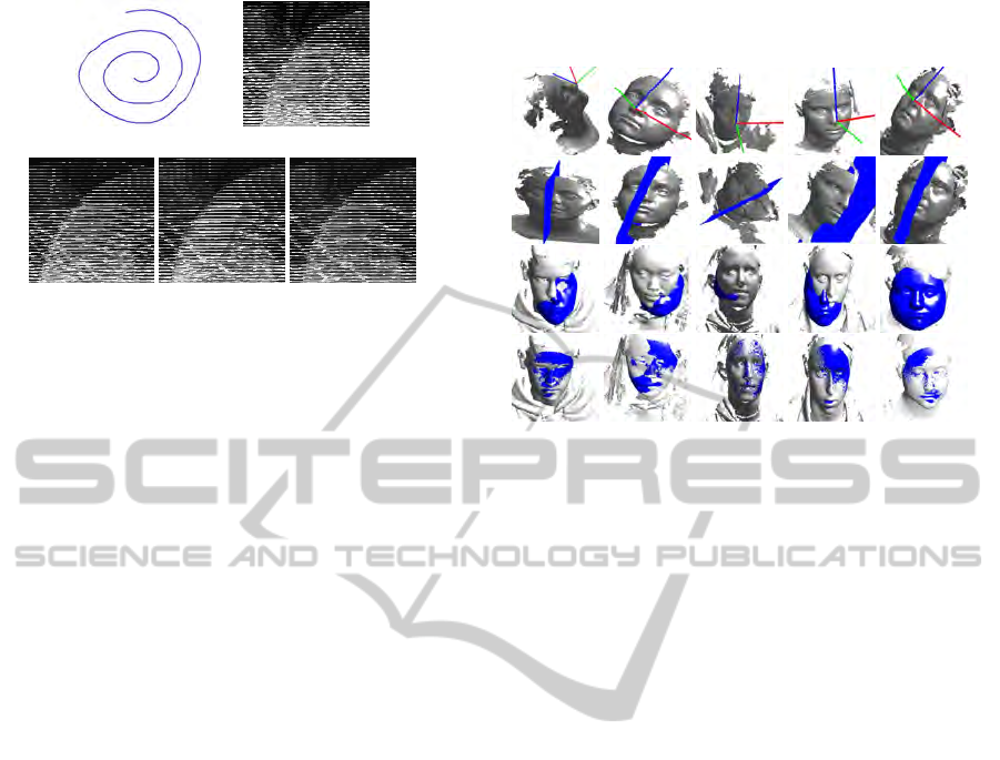
(a) (b)
(c)
Figure 5: a.: A piece of 3D spiral curve emanating from the
nose tip. b: The full spiral curve superimposed on the facial
surface. Facial closed-curves at decreasing sampling rate.
5.4 Face Pose Computation
The computation of the face pose is a critical step to
model based localization and recognition tasks. In
this section, we brief on the details of how our frame-
work is adapted to approximate the face pose of a 3D
facial surface. By face pose, we refer to the coordi-
nate system (O,⃗u,⃗v,⃗w), attached to the face, in which
the origin is the nose tip, and the axis are the gaze di-
rection, the normal to the face symmetry plane, and
the view up direction. In order to determine the face
pose: we begin by grouping all the points that form
the discrete curves C
k
determined in the previous sec-
tion, and simply compute their principal axes via the
standard PCA analysis. Since the curves C
k
inherit the
symmetry property of the facet with respect to face’s
symmetry plane, it is expected that the PCA method
will produce axis that match the face pose to a reason-
ably good extent. In Figure 6.a we depict some exam-
ples of face pose axis plotted on the raw facial scans.
From the face pose, we also derive the face symmetry
plane, having as normal the vector⃗v and including the
nose tip. Some examples of the symmetry plane are
illustrated in Figure 6(2nd row). We assess the pose
estimation methods in two ways, 1) by aligning pairs
of different face scans of the same individuals using
their estimated poses and 2) by comparing the sym-
metry plane computed by our method with symmetry
plan derived from ground truth data. The first experi-
ment was conducted with a group of faces comprising
instances of raw facial scan in neutral expression and
their sad expression counterpart. The facial surface
in this last group are cropped. Figure 6 (3rd and 4th
row) shows some aligned instances. It is clearly ob-
servable that alignments exhibit an acceptable accu-
racy, and thus can be used for a suitable initialization
for the iterative registration algorithms such as the it-
erative closest point method (ICP).
Figure 6: Computation of the face pose (1st row) and deduc-
tion of the face symmetry plane for some face samples (2nd
row). 3rd and 4rth rows:Alignment of cropped instances of
faces exhibiting sad facial expression to their counterparts
raw images in a neutral expressions.
In the second method of assessment, we consider
symmetry plane estimation error as the angle between
the the two normals of the estimated and the actual
planes. We computed the estimation error for a group
of 200 3D face instances (100 neutrals and 100 sads)
and have found a standard deviation error of 2 degree
for a mean error of 0.03 degree, and a maximum error
of 4 degree.
In addition, we also assess the stability of the
Figure 5: a): A piece of 3D spiral curve emanating from
the nose tip. b): The full spiral curve superimposed on the
facial surface. Facial closed-curves at decreasing sampling
rate.
5.4 Face Pose Computation
The computation of the face pose is a critical step to
model based localization and recognition tasks. In
this section, we brief on the details of how our frame-
work is adapted to approximate the face pose of a 3D
facial surface. By face pose, we refer to the coordi-
nate system (O,~u,~v,~w), attached to the face, in which
the origin is the nose tip, and the axis are the gaze di-
rection, the normal to the face symmetry plane, and
the view up direction. In order to determine the face
pose: we begin by grouping all the points that form
the discrete curves C
k
determined in the previous sec-
tion, and simply compute their principal axes via the
standard PCA analysis. Since the curves C
k
inherit the
symmetry property of the facet with respect to face’s
symmetry plane, it is expected that the PCA method
will produce axis that match the face pose to a reason-
ably good extent. In Figure 6.a we depict some exam-
ples of face pose axis plotted on the raw facial scans.
From the face pose, we also derive the face symmetry
plane, having as normal the vector~v and including the
nose tip. Some examples of the symmetry plane are
illustrated in Figure 6(2nd row). We assess the pose
estimation methods in two ways, 1) by aligning pairs
of different face scans of the same individuals using
their estimated poses and 2) by comparing the sym-
metry plane computed by our method with symmetry
plan derived from ground truth data. The first experi-
ment was conducted with a group of faces comprising
instances of raw facial scan in neutral expression and
their sad expression counterpart. The facial surface
in this last group are cropped. Figure 6 (3rd and 4th
row) shows some aligned instances. It is clearly ob-
servable that alignments exhibit an acceptable accu-
racy, and thus can be used for a suitable initialization
for the iterative registration algorithms such as the it-
erative closest point method (ICP).
at the nose tip. Figure 5.b shows an instance of 3D
spiral curve spanning the whole face superimposed
on the original surface. This spiral 3D curve encap-
sulates the facial shape variation at a both local and
global scale. Moreover, since the 3D spiral curve is
attached to the facial surface, it can be augmented to
the normal to the face surface at each of points. We
presume that our facial representation spiral facets is
the only model that encode such facial shape varia-
tion into a single mono-dimensional structure. In the
same vein, we construct a 3D closed curve from each
ring in the spiral facets. We obtain a group of con-
centric curves C
k
,k = 1..N centered at the nose tip.
We can easily control the density of these curves by
a simple subsampling as illustrated in Figure 5.(c).
The
C
k
curves inherit from the spiral facet rings the
iso-geodesic property. Therefore they can be used as
low-cost alternative of the iso-gedesic closed curves
employed in (Samir et al., 2009), which do also re-
quire a mesh regularization.
(a) (b)
(c)
Figure 5: a.: A piece of 3D spiral curve emanating from the
nose tip. b: The full spiral curve superimposed on the facial
surface. Facial closed-curves at decreasing sampling rate.
5.4 Face Pose Computation
The computation of the face pose is a critical step to
model based localization and recognition tasks. In
this section, we brief on the details of how our frame-
work is adapted to approximate the face pose of a 3D
facial surface. By face pose, we refer to the coordi-
nate system (O,⃗u,⃗v,⃗w), attached to the face, in which
the origin is the nose tip, and the axis are the gaze di-
rection, the normal to the face symmetry plane, and
the view up direction. In order to determine the face
pose: we begin by grouping all the points that form
the discrete curves C
k
determined in the previous sec-
tion, and simply compute their principal axes via the
standard PCA analysis. Since the curves C
k
inherit the
symmetry property of the facet with respect to face’s
symmetry plane, it is expected that the PCA method
will produce axis that match the face pose to a reason-
ably good extent. In Figure 6.a we depict some exam-
ples of face pose axis plotted on the raw facial scans.
From the face pose, we also derive the face symmetry
plane, having as normal the vector⃗v and including the
nose tip. Some examples of the symmetry plane are
illustrated in Figure 6(2nd row). We assess the pose
estimation methods in two ways, 1) by aligning pairs
of different face scans of the same individuals using
their estimated poses and 2) by comparing the sym-
metry plane computed by our method with symmetry
plan derived from ground truth data. The first experi-
ment was conducted with a group of faces comprising
instances of raw facial scan in neutral expression and
their sad expression counterpart. The facial surface
in this last group are cropped. Figure 6 (3rd and 4th
row) shows some aligned instances. It is clearly ob-
servable that alignments exhibit an acceptable accu-
racy, and thus can be used for a suitable initialization
for the iterative registration algorithms such as the it-
erative closest point method (ICP).
Figure 6: Computation of the face pose (1st row) and deduc-
tion of the face symmetry plane for some face samples (2nd
row). 3rd and 4rth rows:Alignment of cropped instances of
faces exhibiting sad facial expression to their counterparts
raw images in a neutral expressions.
In the second method of assessment, we consider
symmetry plane estimation error as the angle between
the the two normals of the estimated and the actual
planes. We computed the estimation error for a group
of 200 3D face instances (100 neutrals and 100 sads)
and have found a standard deviation error of 2 degree
for a mean error of 0.03 degree, and a maximum error
of 4 degree.
In addition, we also assess the stability of the
Figure 6: Computation of the face pose (1st row) and deduc-
tion of the face symmetry plane for some face samples (2nd
row). 3rd and 4rth rows:Alignment of cropped instances of
faces exhibiting sad facial expression to their counterparts
raw images in a neutral expressions.
In the second method of assessment, we consider
symmetry plane estimation error as the angle between
the the two normals of the estimated and the actual
planes. We computed the estimation error for a group
of 200 3D face instances (100 neutrals and 100 sads)
and have found a standard deviation error of 2 degree
for a mean error of 0.03 degree, and a maximum error
of 4 degree.
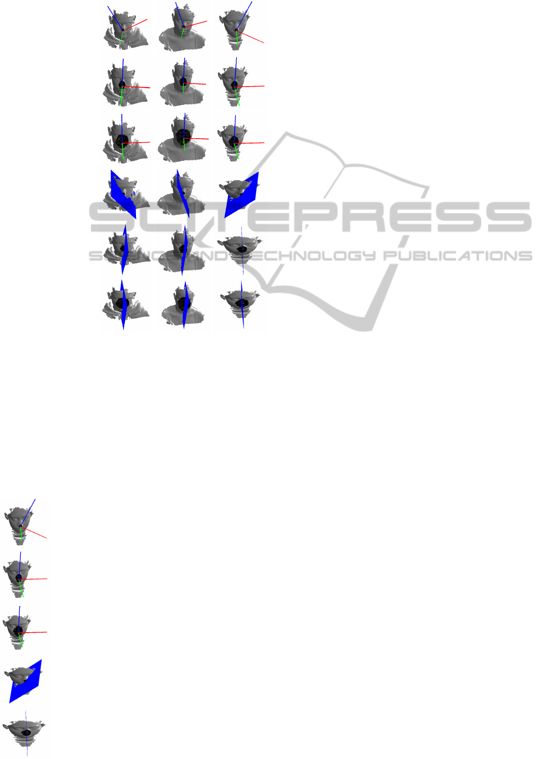
In addition, we also assess the stability of the face
pose estimate against increasing number of rings that
define the faceprint. Here, we consider 100 sample
images, 56 female and 44 male subjects at neutral po-
sitions. For each sample, we compute the face orien-
tation for increasing percentages of the number rings
starting 10% to 90% in steps of 20%. In Figure 7, we
illustrate sample results of the aforementioned exper-
iment. Rows 1 to 3 depict the face orientation with
30%, 50% and 70% of the maximum number rings
and rows 4 to 6 shows the corresponding symmetry
planes for different face samples (columns). As we
can visually notice, the face pose stabilizes nearly at
50% of the maximum number of rings that is required
to describe the facial surface.
To further probe the issue of the stability of face
pose, we construct histograms of the percentage of
number of face images that exhibit stable face orien-
tation against increasing percentage of the number of
rings on distinguished male and female subjects as in
Figure 8. We measure stability in face pose as the
difference in the angular distance between consecu-
tive face pose estimates with increasing rings being
lesser than a predefined threshold (which is 0.15 in
VISAPP 2011 - International Conference on Computer Vision Theory and Applications
36
face pose estimate against increasing number of
rings that define the faceprint. Here, we consider
100 sample images, 56 female and 44 male subjects
at neutral positions. For each sample, we compute
the face orientation for increasing percentages of
the number rings starting 10% to 90% in steps of
20%. In Figure 7, we illustrate sample results of
the aforementioned experiment. Rows 1 to 3 depict
the face orientation with 30%, 50% and 70% of the
maximum number rings and rows 4 to 6 shows the
corresponding symmetry planes for different face
samples (columns). As we can visually notice, the
face pose stabilizes nearly at 50% of the maximum
number of rings that is required to describe the facial
surface.
Figure 7: Stability of the face pose (1-3 columns) and the
corresponding face symmetry plane (4-6 columns) with in-
creasing number of rings (20% rise) on different face sam-
ples (columns)
To further probe the issue of the stability of face
pose, we construct histograms of the percentage of
number of face images that exhibit stable face orien-
tation against increasing percentage of the number of
rings on distinguished male and female subjects as in
Figure 8. We measure stability in face pose as the
difference in the angular distance between consecu-
tive face pose estimates with increasing rings being
lesser than a predefined threshold (which is 0.15 in
our case). It is clear that over 92% of samples need
just 70% of the maximum rings to produce stable face
orientations and nearly 60% of samples need 50% of
the maximum rings to produce stable face pose esti-
mates.
Figure 8: Percentage of face with stabilized face orienta-
tion (y-axis) versus the percentage increase in the number
of rings across male (blue) and female (yellow) samples
5.5 Nose Profile Identification
As the final application of the spiral facets framework,
we describe the problem of nose profile identification.
We define the nose profile as a curve that joins the
nose bridge with the nose tip across the face plane of
symmetry. This curve follows the path of high cur-
vature along the nose, which nearly coincides with
shortest path between these two points. We extend
our framework based on geodesic paths as described
at the end of 4 to identify the nose profile. In effect,
at it is shown in Figure 1.f, geodesic paths that join
neighboring facets, in a given ring of the facet spiral,
to the nose tip, get merged into a common path. This
applies particularly for paths emanating at the cen-
tral forehead where we can clearly observe the con-
vergence of the paths at some level of the nose pro-
file. We draw inspiration from this observation and
use a frequency histogram that accumulates the occur-
rences of the facets at each path. The entries of this
histogram include all the facets crossed by the paths.
Based on this, we propose a nose profile detection
method composed of the following steps: In a first
Figure 7: Stability of the face pose (1-3 columns) and the
corresponding face symmetry plane (4-6 columns) with in-
creasing number of rings (20% rise) on different face sam-
ples (columns).
our case). It is clear that over 92% of samples need
just 70% of the maximum rings to produce stable face
orientations and nearly 60% of samples need 50% of
the maximum rings to produce stable face pose esti-
mates.
face pose estimate against increasing number of
rings that define the faceprint. Here, we consider
100 sample images, 56 female and 44 male subjects
at neutral positions. For each sample, we compute
the face orientation for increasing percentages of
the number rings starting 10% to 90% in steps of
20%. In Figure 7, we illustrate sample results of
the aforementioned experiment. Rows 1 to 3 depict
the face orientation with 30%, 50% and 70% of the
maximum number rings and rows 4 to 6 shows the
corresponding symmetry planes for different face
samples (columns). As we can visually notice, the
face pose stabilizes nearly at 50% of the maximum
number of rings that is required to describe the facial
surface.
Figure 7: Stability of the face pose (1-3 columns) and the
corresponding face symmetry plane (4-6 columns) with in-
creasing number of rings (20% rise) on different face sam-
ples (columns)
To further probe the issue of the stability of face
pose, we construct histograms of the percentage of
number of face images that exhibit stable face orien-
tation against increasing percentage of the number of
rings on distinguished male and female subjects as in
Figure 8. We measure stability in face pose as the
difference in the angular distance between consecu-
tive face pose estimates with increasing rings being
lesser than a predefined threshold (which is 0.15 in
our case). It is clear that over 92% of samples need
just 70% of the maximum rings to produce stable face
orientations and nearly 60% of samples need 50% of
the maximum rings to produce stable face pose esti-
mates.
Figure 8: Percentage of face with stabilized face orienta-
tion (y-axis) versus the percentage increase in the number
of rings across male (blue) and female (yellow) samples
5.5 Nose Profile Identification
As the final application of the spiral facets framework,
we describe the problem of nose profile identification.
We define the nose profile as a curve that joins the
nose bridge with the nose tip across the face plane of
symmetry. This curve follows the path of high cur-
vature along the nose, which nearly coincides with
shortest path between these two points. We extend
our framework based on geodesic paths as described
at the end of 4 to identify the nose profile. In effect,
at it is shown in Figure 1.f, geodesic paths that join
neighboring facets, in a given ring of the facet spiral,
to the nose tip, get merged into a common path. This
applies particularly for paths emanating at the cen-
tral forehead where we can clearly observe the con-
vergence of the paths at some level of the nose pro-
file. We draw inspiration from this observation and
use a frequency histogram that accumulates the occur-
rences of the facets at each path. The entries of this
histogram include all the facets crossed by the paths.
Based on this, we propose a nose profile detection
method composed of the following steps: In a first
Figure 8: Percentage of face with stabilized face orienta-
tion (y-axis) versus the percentage increase in the number
of rings across male (blue) and female (yellow) samples.
5.5 Nose Profile Identification
As the final application of the spiral facets framework,
we describe the problem of nose profile identification.
We define the nose profile as a curve that joins the
nose bridge with the nose tip across the face plane of
symmetry. This curve follows the path of high cur-
vature along the nose, which nearly coincides with
shortest path between these two points. We extend
our framework based on geodesic paths as described
at the end of 4 to identify the nose profile. In effect,
at it is shown in Figure 1.f, geodesic paths that join
neighboring facets, in a given ring of the facet spiral,
to the nose tip, get merged into a common path. This
applies particularly for paths emanating at the cen-
tral forehead where we can clearly observe the con-
vergence of the paths at some level of the nose pro-
file. We draw inspiration from this observation and
use a frequency histogram that accumulates the occur-
rences of the facets at each path. The entries of this
histogram include all the facets crossed by the paths.
Based on this, we propose a nose profile detection
method composed of the following steps: In a first
step we select a ring R that passes through the fore-
head, which generally corresponds the last few rings,
however in order to avoid border effects we choose
the third ring from the last one as illustrated in (Fig-
ure 9.a). The chosen ring R intersects the symmetry
plane at two points within two facets located at the
forehead and chin areas. We then extract a portion
of the ring R keeping the selected facets as the me-
dian as shown in Figure 9.b. In the third step, we
generate a group of geodesic paths converging to the
nose tip. These paths are represented by sequences
of facets joining the two strips to the nose tip (Fig-
ure 9.c). From the two groups of facet sequences S
1
and S
2
we built two histograms that encodes the dis-
tribution of the facets across these paths (Figure 9.d).
From each histogram we extract the two groups of
facets having a score above a certain threshold (Fig-
ure 9.e) and in order to to select the valid group of
facets; we perform a 3D line fitting to the facets’ ver-
tices in each group (Figure 9.f). Finally, we choose
the line producing the least residual error (Figure 9.g)
to correspond to the nose profile. Figure 9.h depicts
some examples of detected nose profiles.
6 CONCLUSIONS AND FUTURE
WORK
In this work, we presented a unified framework for
analyzing and describing 3D facial surface. Our rep-
resentation of 3D facial surface using spiral facets has
THE SPIRAL FACETS - A Unified Framework for the Analysis and Description of 3D Facial Mesh Surfaces
37

step we select a ring R that passes through the fore-
head, which generally corresponds the last few rings,
however in order to avoid border effects we choose
the third ring from the last one as illustrated in (Fig-
ure 9.a). The chosen ring R intersects the symmetry
plane at two points within two facets located at the
forehead and chin areas. We then extract a portion
of the ring R keeping the selected facets as the me-
dian as shown in Figure 9.b. In the third step, we
generate a group of geodesic paths converging to the
nose tip. These paths are represented by sequences
of facets joining the two strips to the nose tip (Fig-
ure 9.c). From the two groups of facet sequences S
1
and S
2
we built two histograms that encodes the dis-
tribution of the facets across these paths (Figure 9.d).
From each histogram we extract the two groups of
facets having a score above a certain threshold (Fig-
ure 9.e) and in order to to select the valid group of
facets; we perform a 3D line fitting to the facets’ ver-
tices in each group (Figure 9.f). Finally, we choose
the line producing the least residual error (Figure 9.g)
to correspond to the nose profile. Figure 9.h depicts
some examples of detected nose profiles.
(a) (b) (c) (d)
(e) (f) (g)
(h)
Figure 9: Nose profile detection. a: Selection of a facet
rings. b:Intersection with the approximate estimation of the
symmetry plane Γ and generation of two stripes. c: Ex-
traction of sequences of facets following the geodesic paths
from the two stripes. to the nose tip. d: For each a group,
a geometric histogram is computed to select facets scoring
large occurrences. e: The two candidate groups of facets (in
blue and yellow in colored images). f: 3D line fitting of two
groups of facets and selection of the one having the lowest
residual error. g: Display of the valid line passing the nose
profile.h: Examples of detected nose profiles.
6 Conclusions and Future Work
In this work, we presented a unified framework for
analyzing and describing 3D facial surface. Our rep-
resentation of 3D facial surface using spiral facets has
resulted in a mechanism that is intrinsic to the face
surface, more simple, compact, generic and compu-
tationally less expensive than other popular represen-
tations. The facet spiral has wide spectrum of appli-
cation that include nose tip detection, frontal face ex-
traction, face shape description, face pose computa-
tion and nose profile identification. In the future, we
plan to explore more deeply the facial shape descrip-
tion aspect. In this context, we plan to investigate how
we can derive from the spiral curves and the concen-
tric close curves, a kind of a ”faceprint” that would
uniquely define the face. We plan also to investigate
further the compactness aspect of the facet spiral, the
spiral-wise ordering of the facets and the topological
constraints in a the facet spiral can exploited to de-
rive a one-dimensional compressed model of the fa-
cial surface.
REFERENCES
Ashbrook, A. P., Fisher, R. B., Robertson, C., and Werghi,
N. (1998). Finding surface correspondance for object
recognition and registration using pairwise geometric
histograms. In Proc European Conference on Com-
puter Vision, pages 674–686.
Berretti, S., Bimbo, A., and Pala, P. (2006). Description and
retrieval of 3d face models using iso-geodesic stripes.
In In Conf. Multimedia Information Retrieval, page
1322.
Bronstein, A., Bronstein, M., and Kimmel, R. (2003). Ex-
pression invariant 3d face recognition. Audio- and
Video-Based Person Authentication, pages 62–70.
Chua, C., Han, F., and Ho, Y. (2000). 3d human face recog-
nition using point signature. In In Conf. on Automatic
Face and Gesture Recognition, pages 233–238.
Colbry, D., Stockman, G., and Jain, A. (2005). Detection of
anchor points for 3d face verification. In Proc. Com-
puter Vision and Pattern Recognition.
Cormen, T. H., Leiserson, C., Rivest, R. L., and Stein., C.
(2001). Introduction to Algorithms, Second Edition.
MIT Press and McGraw-Hill.
F.R., A.-O., Bennamoun, M., and Mian, A. (2008). Integra-
tion of local and global geometrical cues for 3d face
recognition. Pattern Recognition, 41(3):1030–1040.
Frey, P. and Borouchaki, H. (1999). Surface mesh qual-
ity evaluation. International Journal for Numerical
Methods in Engineering, 45(1):101–118.
Heseltine, T., Pears, N., and Austin, J. (2008). Three-
dimensional face recognition using combinations of
Figure 9: Nose profile detection. a: Selection of a facet
rings. b:Intersection with the approximate estimation of the
symmetry plane Γ and generation of two stripes. c: Ex-
traction of sequences of facets following the geodesic paths
from the two stripes. to the nose tip. d: For each a group,
a geometric histogram is computed to select facets scoring
large occurrences. e: The two candidate groups of facets (in
blue and yellow in colored images). f: 3D line fitting of two
groups of facets and selection of the one having the lowest
residual error. g: Display of the valid line passing the nose
profile.h: Examples of detected nose profiles.
resulted in a mechanism that is intrinsic to the face
surface, more simple, compact, generic and compu-
tationally less expensive than other popular represen-
tations. The facet spiral has wide spectrum of appli-
cation that include nose tip detection, frontal face ex-
traction, face shape description, face pose computa-
tion and nose profile identification. In the future, we
plan to explore more deeply the facial shape descrip-
tion aspect. In this context, we plan to investigate how
we can derive from the spiral curves and the concen-
tric close curves, a kind of a ”faceprint” that would
uniquely define the face. We plan also to investigate
further the compactness aspect of the facet spiral, the
spiral-wise ordering of the facets and the topological
constraints in a the facet spiral can exploited to de-
rive a one-dimensional compressed model of the fa-
cial surface.
REFERENCES
Ashbrook, A. P., Fisher, R. B., Robertson, C., and Werghi,
N.(1998). Finding surface correspondance for object
recognition and registration using pairwise geometric
histograms. In Proc European Conference on Com-
puter Vision, pages 674686.
Berretti, S., Bimbo, A. and Pala, P.(2006). Description
and retrieval of 3D face models using iso-geodesic
stripes. In Conf. Multimedia Information Retrieval,
page 1322.
Bronstein, A., Bronstein, M. and Kimmel, R.(2003). Ex-
pression invariant 3D face recognition. Audio-and
Video-based Person Authentication, pages 6270.
Chua, C., Han, F. and Ho, Y.(2000). 3D Human face recog-
nition using point signature. In Conf. on Automatic
Face and Gesture Recognition, pages 233238.
Colbry, D., Stockman, G. and Jain, A.(2005). Detec-
tion of anchor points for 3D face verification. In
Proc.Computer Vision and Pattern Recognition.
Cormen, T. H., Leiserson, C., Rivest, R. L. and Stein.,
C.(2001). Introduction to Algorithms, Second Edition.
MIT Pressand McGraw-Hill.
F. R., A.-O., Bennamoun, M. and Mian, A.(2008). Integra-
tion of local and global geometrical cues for 3D face
recognition. Pattern Recognition, 41(3):10301040
Frey, P. and Borouchaki, H.(1999). Surface mesh qual-
ity evaluation. International Journal for Numerical
Methods in Engineering,45(1):101118.
Heseltine, T., Pears, N. and Austin, J.(2008). Three-
dimensional face recognition using combinations of
surface feature map subspace components. Image and
Vision Computing, 26:382-396
Irfanoglu, M., Gokberk, B. and Akarun, L.(2004). 3D
shape-based face recognition using automatically reg-
istered facial surfaces. In Conf. Pattern Recognition,
volume4, pages 183186.
Kakadiaris, I.(2007). Three-dimensional face recognition in
the presence of facial expressions: An annotated de-
formable model approach. IEEE Transaction on Pat-
tern Analysis and Machine Intelligence,29(4).
Lee, Y., Park, K., Shim, J. and Yi, T.(2003). 3D face recog-
nition using statistical multiple features for the local
depth information. In Conf. Vision Interface, pages
102108.
Lu, X. and Jain, A.(2005). Deformation analysis for 3D
face matching. In IEEE Workshops on Application of
Computer Vision, pages 99104.
Mian, A., Bennamoun, M. and Owens, R.(2007). An effi-
cient multimodal 2D-3D hybrid approach to automatic
face recognition. IEEE Transactions in Pattern Anal-
ysis and Machine Intelligence, 29(11):19271943.
Moreno, A., Sanchez, A. and Martinez, E.(2006). Robust
representation of 3D faces for recognition. Int. Jour-
nal of Pattern Recognition and Artificial Intelligence,
20(8):11591186.
Nair, P. and Cavallaro, A.(2009) 3-d face detection,land-
mark localization, and registration using a point distri-
bution model. IEEE Trans. Multimedia, 1(4):611623.
Pan, G., Wu, Y., Wu, Z. and Liu, W.(2003). 3D face recog-
nition by profile and surface matching. In IEEE/INNS
Conf. on Neural Networks, volume3, pages 21692174.
Piegl, L. and Tiller, W.(2006) The NURBS Book. Springer.
R. Niese, Al-Hamadi, A. and Michaelsi, B.(2007) A novel
method for 3D face detection and normalization. Jour-
nal of Multimedia,2(5):112.
VISAPP 2011 - International Conference on Computer Vision Theory and Applications
38

Romero, M. and Pears, N.(2009). Landmark localisation in
3D face data. In IEEE Conf. on Advanced Video and
Signal Based Surveillance, pages 7378.
Ruiz, M. and Illingworth,J.(2008). Automatic landmark-
ing of faces in 3D-alf. In 5th International Confer-
ence on Visual Information Engineering(VIE2008),
pages4146.
Samir, C., Srivastava, A., Daoudi, M. and Klassen, E.
(2009) An intrinsic framework for Analysis of facial
surfaces. International Journal of Computer Vision,
82(1).
Segundo, M., Queirolo, C., Bellon,O. and Silva, L.(2007).
Automatic 3D facial segmentation and landmark de-
tection. In Proc. 14th Int.Conf. on Image Analysis and
Processing, page431436.
Sethian, J. and Kimmel., R.(1998). Computing geodesic
paths on manifolds. Proc. National Academy of Sci-
ences, 95(15):84318435.
Wang, Y., Tang, X., Liu, J., Pan, G. and Xiao, R.(2008). 3D
face recognition by local shape difference boosting.
In Proc. European Conference on Computer Vision,
ECCV, pages 603616.
Wu, Y., Pan, G. and Wu, Z.(2003). Face authentication
based on multiple profiles extracted from range data.
In Conf. Audio-and Video-Based Biometric Person
Authentication, volume 2688, pages 515522.
Xu, C., Tan, T., Wang, Y. and Quan, L.(2006) Combin-
ing local features for robust nose location in 3D facial
data. Pattern Recognition Letters, 27:14871494.
Xu, C., Wang, Y., Tan, T. and Quan, L.(2004a). Automatic
3D face recognition combining global geometric fea-
tures with local shape variation information. In IEEE
Conf. on Automatic Face and Gesture Recognition,
pages 302307.
Xu, C., Wang, Y., Tan, T. and Quan, L.(2004b) A new at-
tempt to face recognition using eigenfaces. In Asian
Conference on Computer Vision, volume 2, pages
884889.
Xu, D., Hu, P., Cao, W. and Li, H.(2008). 3D face recog-
nition using moment in variants. In IEEE Int. Con-
ference on Shape Modeling and Applications, pages
261262.
THE SPIRAL FACETS - A Unified Framework for the Analysis and Description of 3D Facial Mesh Surfaces
39
