
ONLINE ACTIVITY MATCHING USING WIRELESS SENSOR
NODES
Arie Horst and Nirvana Meratnia
Pervasive Systems, University of Twente, Drienerlolaan 5, Enschede, The Netherlands
Keywords:
Activity matching, Body sensor network, Dynamic time warping.
Abstract:
In this paper, we explore the capability of wireless sensor networks to perform online activity matching for
sport coaching applications. The goal is to design an algorithm to match movements of a trainee and a trainer
online and to find their spatial and temporal differences. Such an algorithm can aid the trainer to better observe
performance of the trainees in group lessons.
We consider fitness-like movements such as those performed in aerobic. We also limit ourselves to only
having one sensor node on the trainer and one sensor node on the trainee, however our algorithm scales
well to more trainees per trainer. We use Sun SPOT sensor nodes and use the accelerometer and gyroscope
sensors to capture the movements. The gravity vector is extracted and improved with a Kalman filter using
the accelerometer and gyroscope data. An automatic segmentation technique is developed that examines the
movement data for rest and activity periods and changes in movement direction. The segmentation and the
movement information are communicated with the node of the trainee where the movements are compared.
We choose to use Dynamic Time Warping (DTW) to perform the spatial and temporal matching of movements.
Because DTW is computationally intensive, we develop an optimized technique and provide feedback to the
trainee. We test all the design choices extensively using experiments and perform a system test using different
test methods to validate our approach.
1 INTRODUCTION
A sport coach is a person who instructs and gives
feedback to other individuals on correctness and their
performance. The sport coach is often called a trainer
and the individuals are often called trainees. Such a
construction is very common in almost all sport do-
mains, such as soccer, tennis, swimming, fitness, etc.
In some of these domains the trainer has to instruct
a group on how to perform a movement. Especially
with large groups it becomes very difficult for the
trainer to keep track of all the trainees and provide
feedback to them. We try to address this problem by
developing a system that assists the trainer with pro-
viding feedback to the trainees about correctness of
their performance using a wireless sensor network.
A wireless sensor network (WSN) is a network
of sensory devices that are wirelessly interconnected
through a radio communication link. All these de-
vices, also refered to as nodes, have some sort of pro-
cessing unit to which sensors are attached and make
perception of some physical quantity possible. Body
sensor networks (BSN) are a special type of WSN in
that they are mostly wireless but do not necessarily
need to realize this via a radio link. BSNs are com-
prised of nodes attached to a body and communicate
with each other either via radio link, the host body or
wires (Lo et al., 2005)(Jones et al., 2008).
Activity recognition is a field of research that in-
vestigates how to accurately detect different activities
a person performs. Examples includes recognizing
activities such as walking, sitting, standing, cooking
and eating(van Kasteren and Krose, 2007)(Tran and
Sorokin, 2008), recognizing gestures from video or
motion sensor data (Whitehead and Fox, 2009)(Yin
and Xie, 2007), or recognizing interaction between
one or more persons or objects (Patterson et al.,
2005)(Wu et al., 2007). The latter is also known as
interaction detection.
Our work examines the use of BSNs to accom-
plish the task of finding spatial and temporal differ-
ences of human body motion between two persons
using inertial sensors in an online and decentralized
manner.
The remainder of this paper is organized as fol-
lows: First related work is discussed in section 2 after
which a detailed description of the system architec-
ture is given in section 3. The components of the ar-
22
Horst A. and Meratnia N..
ONLINE ACTIVITY MATCHING USING WIRELESS SENSOR NODES.
DOI: 10.5220/0003361100220031
In Proceedings of the 1st International Conference on Pervasive and Embedded Computing and Communication Systems (PECCS-2011), pages 22-31
ISBN: 978-989-8425-48-5
Copyright
c
2011 SCITEPRESS (Science and Technology Publications, Lda.)

chitecture are described in more detail in section 4 to
6. Finally the evaluation and conclusion sections con-
clude this paper.
2 RELATED WORK
Activity recognition is a vast research domain that in-
tersects with the domains of image processing, audio
processing and motion sensor data processing.
A method for detection and classification of inter-
action between two persons is presented in the work
of Ruzena Bajcsy et al. (Bajcsy et al., 2009). The goal
of the system is to detect if a classified movement de-
viates from the normal case. To detect these situations
a classification is made by selecting a feature which
has ”minimum distance” to the feature that is tested.
A similar method is used by Davrondzhon Gafurov
et al. (Gafurov and Snekkenes, 2009) for gait recog-
nition using wearable motion sensors. Sensors are
placed on foot, hip, pocket and arm. The Euclidean
distance of the feature vectors and a template is then
compared with a specified threshold. Distance mea-
sures as used by Ruzena Bajcsy et al. (Bajcsy et al.,
2009) and Davrondzhon Gafurov et al. (Gafurov and
Snekkenes, 2009) are simple and generaly cheap in
terms of computation. The main disadvantage of the
method used by the authors is that it is not possible to
detect timing related information.
Yuji Ohgi (OHGI, 2006) uses dynamic time warp-
ing (DTW) to analyse the motion of a swimmer’s arm
stroke and the swing of a golf club in an offline man-
ner on a PC. DTW is a method for finding similarity
in two timeseries that are not necessarily of the same
length and speed and is mostly used in speech recog-
nition. DTW can use any distance meaure to detect
the similarity of two data sets. Furthermore, the two
data sets do not need to be aligned. A disadvantage of
DTW is that it is computationaly intensive.
Marin-Perianu et al. present a lightweight, inex-
pensive and fast incremental algorithm for calculating
cross-correlation (Marin-Perianu et al., 2007). Using
this method it is possible to calculate correlation coef-
ficients on small resource constrained devices such as
wireless sensor nodes. To validate the technique, an
implementation is made that detects if two wireless
sensor nodes move together or separately. The cor-
relation function can detect similarity when the sig-
nals are shifted in time, but not when one signal is
stretched. The optimization made by the authors to
the correlation function introduces another disadvan-
tage. Their method requires very accurate synchro-
nization and cannot detect delays.
Jonathan Lester et al. propose a system that de-
tects if two devices are carried by the same person
(Lester et al., 2004). As a measure for similarity the
coherence function is used which is a measure of sim-
ilarity of two signals in the frequency domain. Using
this technique they can successfully detect if two de-
vices are carried by the same person with detection
rates up to 100%, even when the system is fooled by
two persons walking in step. By using frequency do-
main signals, all timing information is lost and there-
fore, detecting delays is not possible. Additionaly,
a time stretched signal will have very different fre-
quency characteristics than the orignal signal.
3 SYSTEM ARCHITECTURE
In this section a top-down explanation of our system
architecture is given. Nodes placed on the trainer
are designed as Master and the nodes placed on the
trainee are designed as Slave. Furthermore, the map-
ping of the master nodes to the slave nodes is one-to-
one. This means that if a master node is placed on
the left wrist, the slave node should also be placed on
the left wrist and exchange of sample data happens
only between these two nodes. This is defined as a
pair of nodes. More than one slave can be connected
to a master but we will not consider this case. Fig-
ure 1 shows an example of two pairs of nodes placed
on the trainer and the trainee. We choose to place the
sensors on the wrist because at the wrist high acceler-
ations can be measured, while the sensor can still be
attached without causing much discomfort.
(a) Master (b) Slave
Figure 1: Sensor Placement.
The sensor hardware used are the PY530A gyro-
scope and the build-in LIS3L02AQ accelerometer of
the Sun Spot nodes.
Taking the level one step lower to the software
level the following components are required on the
nodes, of which some are master or slave specific.
ONLINE ACTIVITY MATCHING USING WIRELESS SENSOR NODES
23

Sampler
Preprocessing
Segmentation
Communication
(a) Master
Sampler
Preprocessing
Comparing
Communication
Feedback
(b) Slave
Figure 2: Software components.
The software components of our system architecture
are shown in Figure 2.
Sampling is the process of taking data samples of the
sensors. This component is subject to strict and accu-
rate timing as subsequent processing may fail other-
wise. This component is needed on both master and
slave.
Preprocessing involves conditioning and refining the
sensor data and extracting features from the sensor
data. This is done in the preprocessing component
which will be elaborated in section 4.
Segmentation is used to mark the beginning, change
and end of movements in the sensor data stream.
The segmentation component runs only on the mas-
ter node as the trainer is supposed to do it right. The
methods used to accomplish the segmentation are ex-
plained in section 5.
Communication between the master and the slave
node is done wirelessly using the wireless commu-
nication capability of the sensor node.
Comparing of movement data is done on the slave
nodes. The comparison identifies differences in the
amplitude, direction, and timing of movements. The
algorithm used for this process is further elaborated in
section 6.
Feedback is generated from the result of the compar-
ison of movement data and is sent to the base station.
4 PREPROCESSING
In the preprocessing stage, we filter out noise and ex-
tract the gravity vector from the accelerometer data.
To cancel out noise, a technique called oversam-
pling (Watkinson, 1993) can be used. Noise tends to
have the highest concentrations near the sampling fre-
quency because aliases of all higher frequency noise
will show up there. By oversampling this noise
is moved away from the measured frequency band.
The highest frequency of movements is emperically
found to be 10Hz. According to the Nyquist theorem
(Proakis and Manolakis, 2006), data should at least
be sampled twice the time of the highest frequency
component present in the measured signal. Therefore
the sampling frequency should at least be 20Hz. Us-
ing oversampling we choose therefore to sample the
sensor data at 40Hz.
The signal acquired from the accelerometer is the
summation of the accelaration caused by gravity and
the acceleration caused by movement of the device.
This is an undersirable effect when comparing the
movement directions, as how big the measured dif-
ference is then depends on the orientation of both de-
vices.
We choose to extract the gravity vector from the
signal of the accelerometer and then subtract this
gravity signal from the accelerometer signal to ob-
tain the movement vector. Having a movement vector
with gravity eliminated allows better comparison of
the movement direction.
A good first approximation of the gravity vector
can be made using a low pass filter, but this approach
may fail when the sum of the imposed acceleration
and the gravity becomes very small. Here a kalman
filter can help to make a better approximation of the
gravity vector using the turn rates of the gyroscope.
To extract the gravity from the accelerometer data
we choose to apply a low pass filter. A finite impluse
response (FIR) filter is used because of its numeri-
cal stability (Proakis and Manolakis, 2006) and the
fact that it is easy to implement. We have empirically
found that, with regard to our specific type of consid-
ered movements, a cut-off frequency of 0.8Hz gives
excellent results. The gravity vector from this filter is
used as a basis and is further improved using a kalman
filter and the rates of change from the gyroscope.
We choose to use a kalman filter to improve the
estimation of the gravity vector with gyroscope data.
This has the advantage of adding more speed when
the orientation changes too quickly to be followed by
the low pass filter. Also, the gravity extracted by the
low pass filter suffers from overshoot, which will be
damped by the kalman filter when the gyroscope data
disagrees.
PECCS 2011 - International Conference on Pervasive and Embedded Computing and Communication Systems
24

A kalman filter needs a model of the system to
make an estimation of the new state of the system.
The goal is to have a very lightweight kalman filter
with respect to computational requirements. Others
have used kalman filters like the unscented kalman
filter in combination with quaternions to estimate ori-
entation of a rigid body (Kraft, 2003) or a classic
kalman filter with quaternions to estimate angular ve-
locity and position (Yun et al., 2003). Saito H. et al.
(Saito et al., 2009) use in their work a classic kalman
filter to correct joint angles measured from gyroscope
with inclination measured by an accelerometer.
We choose to use the Euler angles coordinate sys-
tem so that a much smaller and simpler steady state
kalman filter can be used. The advantage of a steady
state kalman filter is that it is much more efficient
from a computational demand point of view. The
downside of using the Euler coordinate system is that
it gives singularities at ∼90
◦
. The alternative of a
vector based model would require a rotation matrix
as state transition matrix, which is time dependent. In
that case only an extended kalman filter can be used to
overcome the nonlinearity of the state transition ma-
trix, which is computationaly too demanding.
5 SEGMENTATION
We have empirically found out that the algorithm
to compare the movements needs specific periods of
time to evaluate over. More specifically the best pe-
riods to evaluate are from a beginning to the end of
a movement. To this end an algorithm is needed
that makes a temporal segmentation of the real-time
stream of data, such that each segment will hold at
least one movement. This algorithm will run on the
node of the trainer and will send segmentation events
along with the stream of movement data to the node
of the trainee.
Segmentation techniques can be classified in man-
ual segmentation (Jafari et al., 2007) and automatic
segmentation (Guenterberg et al., 2007)(Guenterberg
et al., 2009)(Chambers et al., 2004). Manual segmen-
tation can be done offline by examining the data or
online using for example a pushbutton. Both of them
are regarded as unacceptable as both the trainee and
the trainer should not be concerned with such a task
and offline segmentation is just not possible as the en-
tire system is to run online in real-time. Guenterberg
et al. (Guenterberg et al., 2007) present an automatic
segmentation technique using windowed standard de-
viation to detect transitions between sitting and stand-
ing states of a human body. Another algorithm also
from Guenterberg et al. uses the signal energy to dis-
tinguish between rest and activity states (Guenterberg
et al., 2009). Chambers et al. (Chambers et al., 2004)
calculate the log likelihood function over a sliding
window. Sharp changes of the likelihood values cor-
respond to change of acceleration value. Others have
used the most simple form of segmentation by using a
sliding window with some overlap (Patel et al., 2009).
All mentioned automatic segmentation techniques
suffer from the problem that stationary signals are de-
tected as rest. As the movements considered in our
scenario can be relatively slow, these methods are not
usable.
Instead we use two separate methods to detect seg-
mentation points. The first method detects whether
the node is moving, and the second method detects
changes in movement direction. The results of these
two methods are then combined to generate segmen-
tation events that will be sent to the slave.
The first method we use takes the magnitude of the
movement vector and the absolute value of the rates
of change of the gyroscope to detect activity or rest.
Three windowed moving average filters, one for the
movement magnitude data and two for the gyroscope
data, are used to smoothen the signals. When at least
one of these moving averages becomes higher than
a certain threshold, the node is considered moving.
When all the averages are lower than a certain thresh-
old, the node is considered not moving. A hysteresis
between these two thresholds is applied to prevent os-
cillation of the movement state.
The second method we use detects abrupt changes
in movement direction. This method evaluates the
dot product of the current movement direction with
a number of movements from recent history, as spec-
ified by Equation 1.
f(i,m,n) =
n
∑
j=m
1−~x
i
·~x
i− j
m > 0 n > m |~x
i
|,|~x
i− j
| > 0.2
(1)
The input vector~x must be normalized so that the
dot product produces the cosine of the angle. The re-
sult of the dot product is then inverted such that two
vectors pointing at the same direction produce zero
and two vectors pointing at opposite direction pro-
duce two. This is evaluated and summed for a number
of vectors from recent history starting at i−m till i−n
such that the result is smoother. We have empirically
found that the magnitude of the vectors (unnormal-
ized) should be bigger than 0.2 to prevent noise trig-
gering the algorithm.
We choose to use a threshold to generate a direc-
tion change event that will be used by the fusion al-
gorithm that will fuse the results of the two methods.
ONLINE ACTIVITY MATCHING USING WIRELESS SENSOR NODES
25

This direction change event is generated only when
Equation 1 becomes higher than a certain threshold.
The two methods are fused using the movement
state and the direction change event. When the state
of movement transits from rest to moving a “Move-
ment Start” segmentation event is generated. A
“Movement Stop” event is generated when the state
of movement transits from moving to rest. When the
movement state is moving, events from the direction
change detection are allowed. In principle both event
types can occur with quick succession. This is pre-
vented by allowing events to occur only when a time-
out has expired since the last event.
6 COMPARING MOVEMENTS
The measurements of the sensors are a representation
of the movements made by the person to which the
sensor node is attached. These measurements are then
transfered from the node of the trainer to the node of
the trainee, where they are compared to find differ-
ences in their movements.
There are many methods to accomplish this, such
as the work of Ryan Aylward et al. (Aylward, 2006)
and Martin Wirz et al. (Wirz et al., 2009) who use cor-
relation as a measure of similarity of movements. The
standard correlation function is improved by making
it incremental by Marin-Perianu et al. in (Marin-
Perianu et al., 2007), who also successfully used it
to measure similarity. Another method is used by
Jonathan Lester et al. (Lester et al., 2004) who used
Coherence to measure similarity.
What all these methods have in common is that
they produce poor results when movements are very
similar and differ only in speed. We choose there-
fore the similarity measure used by Yuji Ohgi (OHGI,
2006), in which dynamic time warping (DTW) is used
to assess the performance of swimmers and golfers.
DTW in its classic form as used by Ohgi is however
not suitable to be used in an online and realtime man-
ner.
To overcome this problem we present an opti-
mized version of the classic DTW in terms of com-
putational requirements. Our new technique, fast in-
cremental dynamic time warping (FIDTW), computes
the optimal shortest warping path and can run on low
power and resource constraint devices. Firstly, we
provide some background on DTW with a mathemat-
ical definition and some notes on related work re-
garding optimization of the conventional DTW algo-
rithm. The remainder of this section will be devoted
to the optimization of the DTW algorithm and we fin-
ish with an evaluation of the choosen algorithm.
6.1 Classic DTW
DTW is a general time alignment and similarity mea-
sure for two temporal sequences and was first intro-
duced by Bellman (Bellman, 2003). Suppose we have
the sequences C(i),1 ≤ i ≤ l,C(i) ∈ R and T( j), 1 ≤
i ≤ l,T( j) ∈ R. These are called a class sequence
and a test sequence, respectively. With these two se-
quences an I × J distance table D(i, j) is constructed
with which similarity can be measured. From the dis-
tance table a warping path W is then calculated which
consists of a set of table elements that defines a map-
ping and an alignment between C(i) and T( j).
W =
w(i(q), j(q))
q = 1,. . . , Q
max(i, j) ≤ Q ≤ I + J − 1
where i(q) ∈ {1, . . . , I} and j(q) ∈ {1, . . . ,J}.
This warping path is restricted by Continuity,
Monotonicity and Endpoint (the path must start at
i(1) = 1, j(1) = 1 and end at i(Q) = I, j(Q) = J). By
summing the local distances over the warping path,
the local distance DTW(C,T) is obtained. One of the
possible choices for finding the best alignment be-
tween the two sequences is to find the warping path
with the minimum DTW distance out of all possible
warping paths. With the following recursive steps, the
optimal warping path can be found and applies local
constraints to the path:
D(i, j) = d(i, j) + min
D(i− 1, j − 1)
D(i, j− 1)
D(i− 1. j)
The recursion is generally initialized as D(1, 1) =
d(1,1) and terminates when i = I and j = J. The time
and space complexity of this approach is O(IJ).
6.2 Fast Incremental Dynamic Time
Warping Algorithm
In this section we explain our optimization made to
the classic DTW algorithm. One should first note
that the aim of the optimization is to make it faster in
terms of required computation time and not necessar-
ily make it less resource hungry in terms of required
memory space. Secondly the optimization should pre-
serve all the characteristics of the classic DTW, which
means that:
• The optimal warping distance should be pre-
served.
• The optimal warping path should be preserved.
• The optimal warping path must be able to be re-
constructed afterwards for analysis.
PECCS 2011 - International Conference on Pervasive and Embedded Computing and Communication Systems
26
11 21 31 41
12 22 32 .. ..
13 23 .. .. .. ..
14 .. .. .. .. ..
.. .. .. .. ..
.. .. .. nk
T
T
(a) Reshaped DTW
11 21 31 41
12 22 32 .. ..
13 23 .. .. .. ..
14 .. .. .. .. ..
.. .. .. .. ..
.. .. .. nk
(b) Appearing stacked arrow form
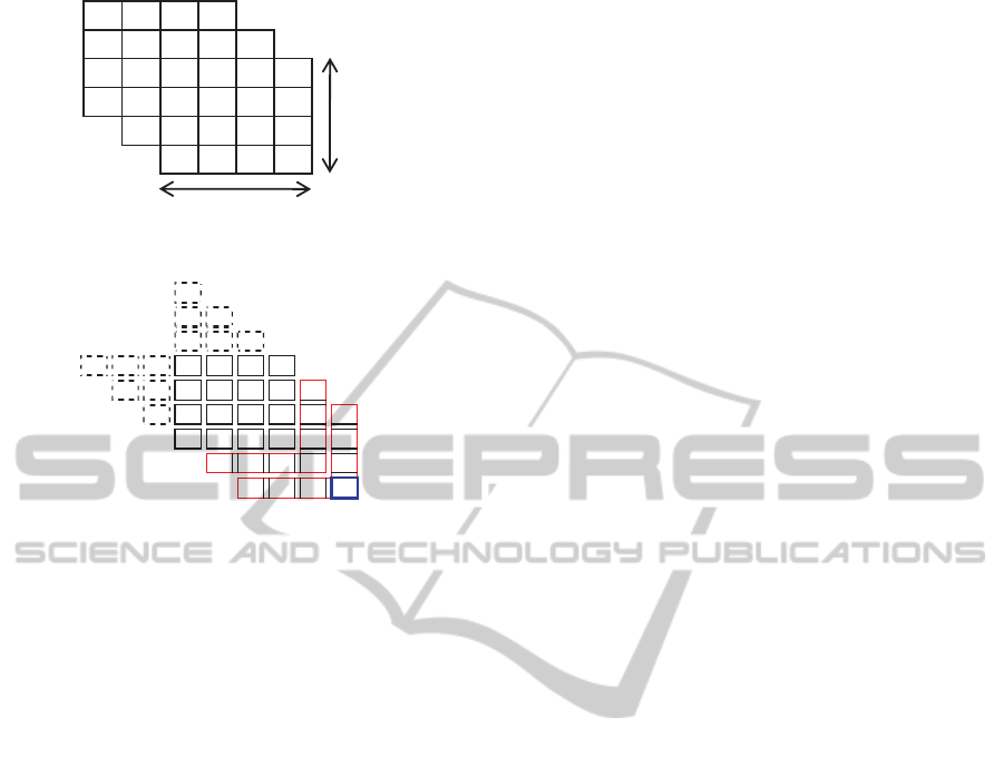
Figure 3: Optimization steps of DTW.
Additionally, the algorithm should work with two
real-time streams that are expected to be synchronized
in time with an negligible error. In case of time syn-
chronized data, it is also observed that:
• The diagonal line from top-left to bottom-right
represents one-to-one allignment of time.
• A warping path that deviates from the diagonal to
the lower left side means that sequence 1 has a
delay compared to sequence 2.
• A warping path that deviates from the diagonal to
the upper right side means that sequence 2 has a
delay compared to sequence 1.
When a maximum positive and negative delay T is
considered, the DTW distance matrix can be reshaped
as shown in Figure 3(a), where the lower left and up-
per right matrix elements that fall outside the delay T
are removed. This is justified as the algorithm is re-
quired to be able to measure delays up to T. The now
appearing shape takes the form of stacked arrows, as
can be seen in Figure 3(b). This arrow shape is from
here on called an arrow object and all the elements
enclosed by the arrow shape directly belong to the ar-
row object. The element of the arrow object which is
emphesized by a blue box is from here on called the
center of the arrow object. The stack form will be ex-
ploited to make the algorithm incremental. The main
construct of the algorithm will then be a list of these
arrow objects. The list is extended at the head until
a maximum length L, after which one arrow object
is removed from the tail everytime an arrow object is
added at the head.
In classic DTW, the accumulated distance matrix
is recomputed everytime the first row or column is re-
moved. One reason for this is because otherwise the
path distance obtained from the accumulated distance
matrix will not be representative anymore. Also from
a practical point of view when dealing with stream
data, values cannot be added into infinity. One possi-
ble way of dealing with this is to recalculate the accu-
mulated distance matrix when needed, but this would
still has ∼O(n
2
) computation time.
It is observed from the classic DTW algorithm
that due to local constraints, only immediate neigh-
bour information is needed to calculate the accumu-
lated distance at a certain point in the matrix. This
means that when a new arrow object is added, the ac-
cumulated distances of this new arrow need only to be
consistent with its successor. However, the accumu-
lated distances are also used to find the shortest DTW
path by traversing backward through the accumulated
distance matrix. This is solved by immediately stor-
ing the neigbor with the lowest accumulated distance
for all the elements of the new arrow object, so that
the shortest DTW path can be found without the ac-
cumulated distances. Now that the accumulated dis-
tances of the new arrow object are calculated and the
reason to keep the accumulated distances consistent
is eliminated, the accumulated distances of the new
arrow object can safely be adjusted. The only valid
method for adjustment is subtraction, because divi-
sion would cause range inconsistency of the distances
of a new arrow object with the accumulated distances
of its successor.
Although it is justified to make the adjustment by
subtracting the lowest accumulated distance in the ar-
row object, only one-eight of the lowest accumulated
distance is subtracted to better preserve the scale that
these distances represent. This is required for the
Flexible Endpoint algorithm that will be explained in
section 6.2.1.
To derive the computational complexity of adding
a new arrow object we assume one penalty for com-
puting the distance of an element and three penalties
for computing the accumulated distance of an ele-
ment. This needs to be computed for T elements of an
arrow object (see Figure 3(b)) so that the total com-
putational complexity becomes ∼O(6T). There is no
penalty for computing the neighbour with lowest ac-
cumulated distance because this is already computed
when the accumulated distance of an element is cal-
culated, and requires only extra storage per element
of an arrow object. However, traversing backwards
along the warping path becomes slightly faster. The
ONLINE ACTIVITY MATCHING USING WIRELESS SENSOR NODES
27
distance of a warping path is now obtained by adding
up all the distances when traversing backward along
the warping path, as the elements of the accumulated
distance matrix do not represent real distances any-
more.
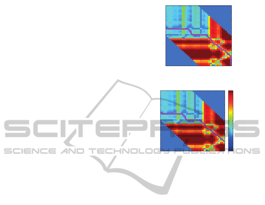
6.2.1 Flexible Endpoint
While testing the algorithm, we found out that the al-
gorithm may find a warping path with a very high dis-
tance although the two signals were very similar but
slightly delayed. An example of such a case is shown
in Figure 4(a). From this figure it can be seen that the
distance in the area at the bottom right corner is very
large. This is because the movement of the trainer is
finished at this point, but the trainee did not. From
Figure 4(a) it can be seen that there is an area with
very high distances at the bottom right corner. The
DTW path has to cross this area to reach the bottom
right corner, which gives the wrong impression that
the two movements are very distant.
This problem is solved by allowing flexible end-
point at the start of the path at the bottom right corner.
The bottom right corner is the head of the list of ar-
row objects of the FIDTW algorithm. Evaluation of
the shortest DTW path starts at the head of the list of
arrow objects at the center of the arrow (the blue box
in Figure 3(b)). A flexible endpoint algorithm there-
fore finds a more suitable start position in this arrow
object. Flexible endpoint algorithms are widely used
with DTW. It is unclear who first proposed the use of
flexible endpoints, but probably one of the first to pro-
pose such a technique is Haltsonen (Haltsonen, 1985).
We chooseto accomplish the task by taking the ac-
cumulated distance of the center of the arrow object
as reference and find an accumulated distance in the
arrow that is at least 25% or lower than the reference
with a 1% penalty for every element it is further away
from the reference. An example of a path produced
with the flexible endpoint algorithm is shown in Fig-
ure 4(b). The path is identical, except in the bottom
right corner, where the path produced with the flexi-
ble endpoint approach does not end in the far bottom
right corner.
6.2.2 Distance Calculation
The distances for the DTW distance matrix are a com-
bination of distance measures of multiple sources.
The used sources are the magnitude of the movement,
the direction of the movement and the change of ori-
entation as measured by the gyroscope. The distance
between the movement magnitudes are calculated us-
ing the squared Euclidean distance function (Equation
2). A magnitude is only one value such that equation
5 10 15 20 25 30 35 40
5
10
15
20
25
30
35
40
(a) Classic DTW path
5 10 15 20 25 30 35 40
5
10
15
20
25
30
35
40
0.0001
0.000316228
0.001
0.00316228
0.01
0.0316228
0.1
0.316228
1
(b) Flexible endpoint
Figure 4: DTW paths.
2 simplifies to Equation 3
d(p, q) =
n
∑
i=1
(p
i
− q
i
)
2
(2)
d(p, q) = (p− q)
2
(3)
The changes of orientation measured by the gyro-
scope are linear, therefore the Euclidean distance can
safely be used as a distance measure. For a two di-
mensional gyroscope n becomes 2 in Equation 2.
The distance between the direction of movements
is measured using Equation 4, which calculates the
angle between two vectors by evaulating the arc co-
sine of the dot product of the two normalized move-
ment vectors. This distance measure is only evaluated
when the magnitude of both vectors is large enough,
because the noise becomes more dominant when the
magnitude of the movement is small.
d(~x
1
,~y
1
) = arccos(~x
1
·~y
1
) |~x
1
|,|~y
1
| > 0.2 (4)
These three distances are then combined by mul-
tiplying them with a weight factor and then adding
them up to one distance measure (Equation 5). The
weight factors facilitate the calibration of the system.
d
combined
= W
magn
∗ d
magn
+
W
dir
∗ d
dir
+W
orient
∗ d
orient
(5)
PECCS 2011 - International Conference on Pervasive and Embedded Computing and Communication Systems
28

6.3 Path Analysis
With the temporal segmentation information an anal-
ysis of the path produced by the FIDTW algorithm
can be made. From this analysis appropiate feedback
can be given to the trainee. From the DTW path a
number of statistical data can be extracted. Figure
5 depicts a typical path produced by our FIDTW al-
gorithm when two movements are very similar. The
diagonal elements from bottom-right to top-left of
the distance matrix represent perfect time alignment.
With respect to the stated direction of the diagonal
line, a deviation to the right represents a positive de-
lay and deviation to the left represents a negative de-
lay. Small differences between two movements may
already cause small delays, often shifting back and
forth from positive to negative delays. Therefore we
use the mean of the delays in a segment.
The DTW path distance represents the similarity
of two signals. This distance also depends on the
length of the path and is therefore normalized by the
path length. The smaller the path distance the more
similar the movements are.
When the path distance is high the two movements
are detected as dissimilar. The cause of the high dis-
tance needs to be found. This information is, for
every element, stored in the DTW distance matrix.
Then during path analysis this information is recov-
ered from the distance matrix such that it can be used
as feedback.
5 10 15 20 25 30 35 40
5
10
15
20
25
30
35
40
0.0001
0.000316228
0.001
0.00316228
0.01
0.0316228
0.1
0.316228
1
Figure 5: Example DTW path.
7 EVALUATION
We assess the correctness of our online matching
technique using three different methods:
1. The node of the trainer and the node of the trainee
are both placed on the same wrist of one person.
This test should always label the movements as
correct and not delayed.
2. The node of the trainer is placed on one wrist and
the node of the trainer on the other wrist of one
person. With this test there is already no real
ground truth anymore, other than the feeling of
the person that he made the same movement with
both arms.
3. One person wears the master node on the right
wrist while another person wears the slave node
on the right wrist.
The feedback which is sent from the slave node
holds information about the incorrectness of the
movement, the timing and the cause of the incorrect-
ness. The measure for incorrectness is the distance
between the movements measured using the FIDTW
algorithm. The timing is either an earlyness or a late-
ness in the form of a positive or negative average de-
lay. When the distance is larger than a certain thresh-
old, the movement can be regarded as incorrect.
7.1 Test Methodology
For the three test methods a test set of three tests, men-
tioned in Table 1, is defined. This test set consists of
repetitive distinct movements. For every test in the set
there is one movement repetition defined for the mas-
ter node and multiple variations of this movement for
the slave node. These variations differ in direction, in
amplitude and in timing.
Table 1: Test set.
Test Description
1 Stretched arm swings 90 degrees from horizon-
tal to vertical position in the upward direction
and goes back to the horizontal position.
2 Right arm is stretched away from the body to
the right in a horizontal straight line and then
attracted to the body again.
3 Right arm is stretched away from the body in
the upward direction in a vertical straight line
and moves back towards the body again.
7.2 Summary of Results
All tests are made indoors in a room with good radio
reception to prevent link losses corrupting the mea-
surements. For method 1 all tests are repeated three
times, and for methods 2 and 3 the tests are repeated
two times. The duration of every test is about 20 sec-
onds, during which the movement is repeated contin-
uously without rest. This results in about ten repeated
identical movements, which should be detected and
classified by the algorithm. The classification can be
either correct or incorrect. The correct classification
rate then is the number of correctly classified move-
ments over the total number of movements presented
ONLINE ACTIVITY MATCHING USING WIRELESS SENSOR NODES
29

in percentage for each method of testing.
In the tests with method 1 the master and slave
nodes are both attached to the same wrist of the per-
former. Therefore, there are no variations for the slave
node and the expected result is that the algorithm clas-
sifies all the movements as identical. We repeated all
tests three times and obtained a correct detection rate
of 99%.
In the tests with method 2 the master and slave
nodes are attached to two wrists of one performer. Us-
ing clear differences in movements we asses if the al-
gorithm correctly classifies the movements. The cor-
rect detection rate for identical movements, 45
◦
di-
rection difference, 90
◦
direction difference, 0.5 sec-
ond timing difference and 30cm distance difference
are respectively 97%, 84%, 89%, 90% and 92%. We
observed that direction differences are undetectable
by the sensor nodes in this test. When the orienta-
tion of the sensor node would be known, this problem
could be solved. However, obtaining an orientation is
not easily accomplished.
In the tests with method 3 the master and slave
nodes are attached to the right wrist of two perform-
ers. With this test we asses the real life performance
of our algorithm. The correct detection rate for iden-
tical movements, 90
◦
direction difference, 0.5 second
timing difference and 30cm distance difference are re-
spectively 86%, 83%, 60%, and 40%.
8 CONCLUSIONS AND FUTURE
WORK
We presented an online and distributed activity
matching algorithm using wireless sensor networks.
Our experimental results show a high detection accu-
racy for identical movements, although it shows high
sensitivity on how movements are performed
The most important open issue is to make the al-
gorithm work reliably in detecting movement differ-
ences between two persons. The low reliability at
present is partly caused by the orientation issue, but
also because the algorithm is over sensitive to subtle
movement differences. The solution to this problem
may be found in using other distance measures and
other sensors.
A second open issue is the orientation problem.
Due to this problem, the sensor orientation must
closely match when attached to the wrist, but also dur-
ing movements the orientation must closely match.
This makes testing with two persons hard and more
unreliable. The problem maybe solved by using dif-
ferent sensors that allow to measure all degrees of
freedom, such that the orientation can be derived.
This is not an easy task and may not work reliably
or fast enough to be used for this application.
The gravity detection may be further improved by
using quaternions instead of euler angles, such that
singularities are avoided. This will make the Kalman
filter more complex, but will improve the reliability
of the estimation.
Future work will also require an extensive evalua-
tion with more users.
REFERENCES
Aylward, R. (2006). Sensemble: A wireless, compact,
multi-user sensor system for interactive dance. In
Proc. of NIME 06, pages 134–139.
Bajcsy, R., Borri, A., Benedetto, M. D. D., Giani, A.,
and Tomlin, C. (2009). Classification of physical in-
teractions between two subjects. Wearable and Im-
plantable Body Sensor Networks, International Work-
shop on, 0:187–192.
Bellman, R. E. (2003). Dynamic Programming. Dover Pub-
lications, Incorporated.
Chambers, G. S., Venkatesh, S., West, G. A. W., and Bui,
H. H. (2004). Segmentation of intentional human ges-
tures for sports video annotation. In MMM ’04: Pro-
ceedings of the 10th International Multimedia Mod-
elling Conference, page 124, Washington, DC, USA.
IEEE Computer Society.
Gafurov, D. and Snekkenes, E. (2009). Gait recognition
using wearable motion recording sensors. EURASIP
J. Adv. Signal Process, 2009:1–16.
Guenterberg, E., Bajcsy, R., Ghasemezadeh, H., and Jafari,
R. (2007). A segmentation technique based on stan-
dard deviation in body sensor networks. In Dallas-
EMBS ’07: Proceedings of the IEEE Dallas Engineer-
ing in Medicine and Biology Workshop. IEEE.
Guenterberg, E., Ostadabbas, S., Ghasemzadeh, H., and
Jafari, R. (2009). An automatic segmentation tech-
nique in body sensor networks based on signal energy.
In BodyNets ’09: Proceedings of the Fourth Interna-
tional Conference on Body Area Networks, pages 1–7,
ICST, Brussels, Belgium, Belgium. ICST (Institute for
Computer Sciences, Social-Informatics and Telecom-
munications Engineering).
Haltsonen, S. (1985). Improved dynamic time warping
methods for discrete utterance recognition. Acoustics,
Speech and Signal Processing, IEEE Transactions on,
33(2):449 – 450.
Jafari, R., Li, W., Bajcsy, R., Glaser, S., and Sastry, S.
(2007). Physicalactivity monitoring for assisted living
at home. In BSN ’07: Proceedings of the 4th Interna-
tional Workshop on Wearable and Implantable Body
Sensor Networks, pages 213–219, Berlin, Heidelberg.
Springer.
Jones, V., in ’t Veld, R. H., Tonis, T., Bults, R., van,
B. B., Widya, I., Vollenbroek-Hutten, M., and Her-
mens, H. (2008). Biosignal and context monitoring:
PECCS 2011 - International Conference on Pervasive and Embedded Computing and Communication Systems
30

Distributed multimedia applications of body area net-
works in healthcare. In Proceedings IEEE 10th Work-
shop on Multimedia Signal Processing, 2008, pages
820–825, Cairns, Australia. IEEE Signal Processing
Society.
Kraft, E. (2003). A quaternion-based unscented kalman fil-
ter for orientation tracking. In Proceedings of the Sixth
International Conference on Information Fusion, vol-
ume 1, pages 47–54.
Lester, J., Hannaford, B., and Borriello, G. (2004). Are you
with me? using accelerometers to determine if two
devices are carried by the same person. In In Proceed-
ings of Second International Conference on Pervasive
Computing (Pervasive 2004, pages 33–50.
Lo, B. P. L., Thiemjarus, S., King, R., and zhong Yang,
G. (2005). Body sensor network - a wireless sensor
platform for pervasive healthcare monitoring. In Ad-
junct Proceedings of the 3rd International conference
on Pervasive Computing (PERVASIVE’05, pages 77–
80.
Marin-Perianu, R., Marin-Perianu, M., Havinga, P., and
Scholten, H. (2007). Movement-based group aware-
ness with wireless sensor networks. In PERVA-
SIVE’07: Proceedings of the 5th international confer-
ence on Pervasive computing, pages 298–315, Berlin,
Heidelberg. Springer-Verlag.
OHGI, Y. (2006). Mems sensor application for the motion
analysis in sports science. ABCM Symposium Series
in Mechatronics, 2:501–508.
Patel, S., Mancinelli, C., Healey, J., Moy, M., and Bonato,
P. (2009). Using wearable sensors to monitor physical
activities of patients with copd: A comparison of clas-
sifier performance. Wearable and Implantable Body
Sensor Networks, International Workshop on, 0:234–
239.
Patterson, D. J., Fox, D., Kautz, H., and Philipose, M.
(2005). Fine-grained activity recognition by aggregat-
ing abstract object usage. In ISWC ’05: Proceedings
of the Ninth IEEE International Symposium on Wear-
able Computers, pages 44–51, Washington, DC, USA.
IEEE Computer Society.
Proakis, J. G. and Manolakis, D. G. (2006). Digital Signal
Processing Principles Algorithms and Applications.
Prentice hall (4th ed).
Saito, H., Watanabe, T., and Arifin, A. (2009). Ankle
and knee joint angle measurements during gait with
wearable sensor system for rehabilitation. In World
Congress on Medical Physics and Biomedical Engi-
neering, pages 506–509, Berlin, Heidelberg. Springer.
Tran, D. and Sorokin, A. (2008). Human activity recogni-
tion with metric learning. In ECCV ’08: Proceedings
of the 10th European Conference on Computer Vision,
pages 548–561, Berlin, Heidelberg. Springer-Verlag.
van Kasteren, T. and Krose, B. (2007). Bayesian activity
recognition in residence for elders. In Intelligent En-
vironments, 2007. IE 07. 3rd IET International Con-
ference on, pages 209–212.
Watkinson, J. (1993). The Art of Digital Audio.
Butterworth-Heinemann, Newton, MA, USA, 2nd
edition.
Whitehead, A. and Fox, K. (2009). Device agnostic 3d ges-
ture recognition using hidden markov models. In Fu-
ture Play ’09: Proceedings of the 2009 Conference on
Future Play on @ GDC Canada, pages 29–30, New
York, NY, USA. ACM.
Wirz, M., Roggen, D., and Troster, G. (2009). Decentral-
ized detection of group formations from wearable ac-
celeration sensors. Computational Science and En-
gineering, IEEE International Conference on, 4:952–
959.
Wu, J., Osuntogun, A., Choudhury, T., Philipose, M., and
Rehg, J. M. (2007). A scalable approach to activity
recognition based on object use. In In Proceedings
of the International Conference on Computer Vision
(ICCV), Rio de.
Yin, X. and Xie, M. (2007). Finger identification and hand
posture recognition for human-robot interaction. Im-
age and Vision Computing, 25(8):1291 – 1300.
Yun, X., Lizarraga, M., Bachmann, E., and McGhee, R.
(2003). An improved quaternion-based kalman filter
for real-time tracking of rigid body orientation. In In-
telligent Robots and Systems, 2003. (IROS 2003). Pro-
ceedings. 2003 IEEE/RSJ International Conference
on, volume 2, pages 1074–1079.
ONLINE ACTIVITY MATCHING USING WIRELESS SENSOR NODES
31
