LEARNING OBJECT DETECTION USING

MULTIPLE NEURAL NETWORKS

Ignazio Gallo and Angelo Nodari

University of Insubria, Dipartimento di Informatica e Comunicazione, Varese, Italy

Keywords:

Object detection, Neural networks, Multiple neural networks.

Abstract:

Multiple neural network systems have become popular techniques for tackling complex tasks, often giving

improved performance compared to a single network. In this study we propose an innovative detection al-

gorithm in image analysis using a multiple neural network approach where many neural networks are jointly

used to solve the object detection problem. We use a group of networks conﬁgured with different parameters

and features, then combines them in order to obtain new networks. The topology of the set of neural networks

is statically conﬁgured as a tree where the root node produces in output the detection map. This work repre-

sents a preliminary study through which we want to move from detection to segmentation and recognition of

objects of interest. We have compared our model with other detection algorithms using a standard dataset and

the results are encouraging. The results highlight the advantages and problems that will guide the evolution of

the proposed model.

1 INTRODUCTION

Object detection is an important task in computer vi-

sion, it is a critical part in many applications such

as content based image retrieval, understanding of a

scene, automatic annotations, etc. However it is still

an open problem due to the heterogeneity of some

classes of objects to be detect and the complexity of

the background in some images. Many works avail-

able in literature work well only on certain categories

of images and fall on others. In this paper we propose

a method capable of maintaining the same accuracy

on different types of data.

Usually the object of interest in a digital image is

detected ﬁnding the bounding box which surround the

object. The strength of this work consist in the detec-

tion of the object in a cognitive manner, locating the

object through the use of a segmentation process. De-

tection and segmentation of an object in a single step

is certainly a more complex and difﬁcult operation in-

stead of detect an object and perform a segmentation

in a second step. In this work we use only the detec-

tion phase of our algorithm in order to compare the

results with other object detection techniques despite

the algorithm presented performs also a segmentation

of the object of interest.

In literature there are many object detection ap-

proaches which can be classiﬁed as bag of words

model (Csurka et al., 2004; Fei-fei, 2005; Schmid,

2006), parts and structure models (Fischler and

Elschlager, 1973; Fergus et al., 2003; Crandall et al.,

2005), discriminative methods (Bouchard and Triggs,

2005; Zhu and Yuille, 2006) and combined segmen-

tation and recognition methods (Leibe and Schiele,

2003; Todorovic and Ahuja, 2006). In this work,

choosing to work with neural networks that combine

the segmentation and recognition, we can classify our

algorithm in the latter object recognition approach.

The model proposed in this study, like other works

which propose biologically inspired systems (Riesen-

huber and Poggio, 1999; Serre et al., 2005), is in-

spired by the human visual perception system. In

fact, analyzing how the visual system works, a neu-

ron n of the visual cortex receives a bottom-up sig-

nal X from the retina (lower-level-input) and a signal

M from an object-model-concept m (top-down prim-

ing signal). The neuron n is activated if both signals

are strong enough. The visual perception uses many

levels in the transition from the retina to object per-

ception. By analogy, we propose a Multi-net system

(Sharkey, 1999) based on a tree-structure where leaf

nodes represent the bottom-up signal extracted from

the input image. The intermediate levels nodes repre-

sent the knowledge of the previous experience, going

in the direction of the root node.

In this paper, unlike for Perceptron Decision

131

Gallo I. and Nodari A..

LEARNING OBJECT DETECTION USING MULTIPLE NEURAL NETWORKS.

DOI: 10.5220/0003328301310136

In Proceedings of the International Conference on Computer Vision Theory and Applications (VISAPP-2011), pages 131-136

ISBN: 978-989-8425-47-8

 2011 SCITEPRESS (Science and Technology Publications, Lda.)

Tree (Utgoff, 1988) which has a similar structure to

the method presented here, the prediction of a trained

network can become an input feature of a second neu-

ral model. Starting from the root node of a tree of

neural networks, the training process is propagated to

the leaf nodes of the tree (networks that depend only

by simple features). During the detection phase, each

node gives its generated map to its parent node un-

til the map produced by the root node. Each node

reads its information through a sliding window that

receives all the input features. Neural networks are

trained on the same set of training images and the

prediction of each of them is combined in order to

improve their generalization attitude. The peculiarity

of the proposed model is that each level of the tree is

guided by the same rules: for each node the percep-

tion of small and particular features or the knowledge

of more abstract and complex concepts is performed

by the same mechanism described above, but using a

different node conﬁguration.

2 THE PROPOSED METHOD

In this section we present our model called Multi-Net

for Object Detection (MNOD). The MNOD model

consists of a tree of single networks C

(F), where n

is the node identiﬁer, P corresponds to all the param-

eters from which the network conﬁguration depends

and F represents the set of input features.

Each neural network C

uses a particular set of

parameters P such as training epochs, number of neu-

rons in the input layer, number of neurons in the hid-

den layer, etc.. The set of features F can be directly

extracted from the input images (such as edges, color,

etc...) or they can be the result of other neural models

previously trained on the same training set. Fig-

ure 1 shows an example of a generic MNOD.

Each node C

produces in output a map where the

pixels containing higher values identify the objects of

interest. As said in (Sharkey, 1999) it is possible to

diversify a node C

changing network initialization

conditions, topologies, training algorithms and train-

ing data. Here, we investigate only in changing the

network topology considering the set of parameters

P. The main parameters associated which each node n

are P

= {I

}, where I

represents the re-sized im-

age dimension and W

is the sliding window dimen-

sion. The structure of a single node used in this work,

is showed in Figure 2. It consist in a Multi-Layer Per-

ceptron (MLP) which receives the input values from a

sliding window for each feature conﬁgured. We cre-

ate an image for each feature and all these images

are re-sized to the pre-deﬁnite dimension. By using

different combinations of these two parameters it is

possible to construct models specialized in the recog-

nition of a speciﬁc element of interest in a particular

scale. This concept is typical of Multi-net systems

which use a “modular combination” of the neural net-

works (Sharkey, 1999). In this case the main prob-

lem is divided into sub-tasks and then it is possible to

obtain a solution by combining different modules, or

neural networks.

During the training phase all the input and output

images of a node n are re-sized to the same size I

∈

and from all the gray values in the sliding window

we construct the input and desired output (as showed

in Figure 2).

A single node in the proposed model can be

trained or used directly in generalization unless it re-

ceives in input the output of another neural model (see

for example the nodes C

e C

in the Figure 1).

Otherwise (see, for example nodes C

e C

in the

Figure 1) we ﬁrst need to train and then to use the

networks of child nodes. For more details on the al-

gorithms used for training the model see the Algo-

rithm 1 and the Figure 2, while for generalization see

Algorithm 2 and Figure 2.

Algorithm 1: Creating the training set for a node C

(F).

Require: Let D = {(I

out

),...,(I

out

)} the set

of images pairs;

1: for all (I

out

) ∈ D do

2: create images F

,...,F

from I

3: if ∃F

which is the output of a child node C

then

4: execute this algorithm for the node C

5: train the node C

6: use the trained model to create the image F

7: end if

8: Resize F

,...,F

and I

out

at dimension I

∈ P

9: Create an input and an output pattern for each

position of the sliding window W

∈ P (step s

depends by the image size I

)

10: end for

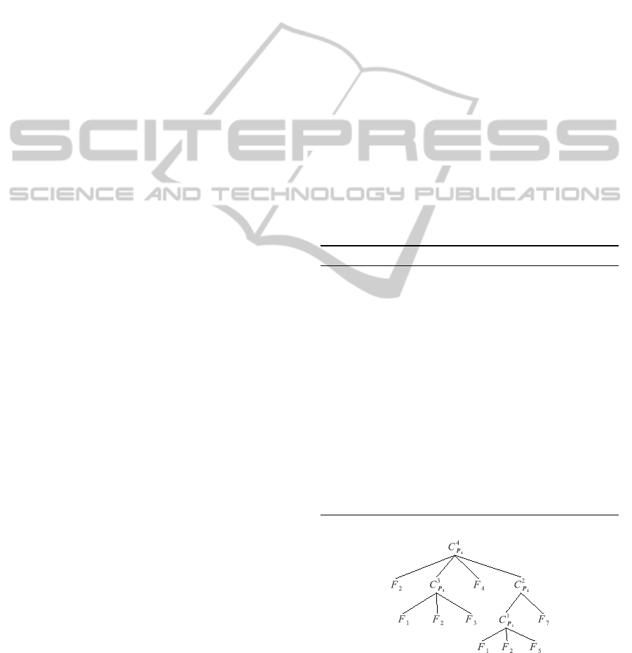
Figure 1: Generic structure of the proposed MNOD model.

The nodes C

represent the supervised neural models which

receive their input directly from the input features, the nodes

are the feature maps extracted from the input images.

VISAPP 2011 - International Conference on Computer Vision Theory and Applications

132

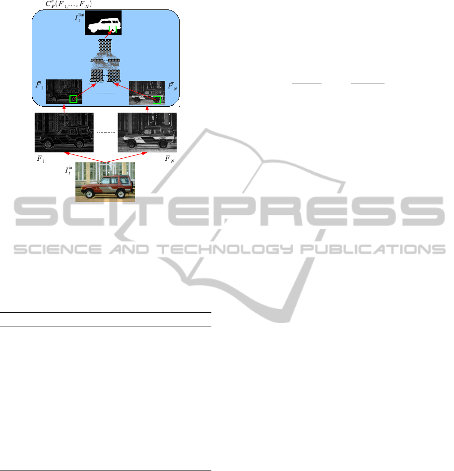
Figure 2: Generic structure of a node C

,... ,F

). The

features F

,... ,F

are created from each input images I

All the features images are re-sized in according to the pa-

rameter I

∈ P in

,... ,

. The output image I

out

is hand-

segmented and contains higher values for the pixels belong-

ing to the objects of interest. The input patterns of the neural

model are generated using a sliding window of size W

∈ P

which reads from the re sized images

,... ,

, while the

desired output is derived from the re sized output image

out

Algorithm 2: Generalization of a single node C

(F).

Require: an image I

to pass in input to the trained

model

1: create F = {F

,...,F

} from I

for the node C

2: if ∃F

which is the output of a child node C

then

3: apply this algorithm to the node C

4: end if

5: Resize F

,...,F

at dimension I

∈ P

6: Create an input pattern for each position of the

sliding window W

∈ P (step 1)

7: Store output predictions of node C

(F)

8: Compose the output image using the average ac-

tivation values for each pixel

3 EXPERIMENTS

In this study, two types of experiments were con-

ducted to analyze different aspects of the proposed

model. We ﬁrst analyzed the main parameters of the

MNOD models and its generalization attitude. Fi-

nally, we tried to compare our model with the results

obtained by other methods using a standard dataset.

The two variables of interest to measure the ac-

curacy of an object detection system, are the num-

ber of correct detections that we want to maximize,

and the number of false detections that we want to

minimize. When an object detection system is really

used, we are interested to know how many objects

have been identiﬁed, and how often the items found

are false. This compromise can be captured by study-

ing the Precision-Recall curve (or PR-curves), where

P =

correct

actual

, R =

correct

possible

(1)

stating that correct is the number of objects correctly

detected by the system, actual is the total number of

objects recognized by the system, possible is the total

number of objects we expected from system. A Pre-

cision equals to 1.0 means that each detected object is

correct, but tells us nothing about the objects that have

not been found. A high Precision value ensures that

there are few false positives. A Recall measure equals

to 1.0 tells us that each object was correctly identi-

ﬁed, but tells us nothing about how many other items

were incorrectly matched. A measure that usually is

used to summarize Precision and Recall values is the

F-measure F1 = 1/(λP + (1 − λ)R) setting λ = 0.5.

Average Precision (AP) is another measure that ap-

proximates the area under the PR-curve and that, for

its readability, is usually used to compare different ob-

ject detection algorithms. For more details on these

measures and how an object is considered correctly

detected see (Everingham et al., 2005).

3.1 Analysis of Key Parameters

In this experiment we analyzed the behavior of the

MNOD model varying its key parameters. In partic-

ular, we analyzed the inﬂuence of the image size I

and the sliding window size W

parameters, applied

to nodes (or networks) conﬁgured with different fea-

tures.

The dataset used here contains real images of cars

viewed from different viewpoint: side, rear, top, front,

partial (see some examples in Figure 4). In particular,

we used the dataset called TU-Graz cars contained in

VOC2005 (Everingham et al., 2005).

For this experiment we used a limited set of fea-

tures that highlight some information on color and

high frequencies available in the images. In partic-

ular, we used the features Saturation (Sa), Hue (Hu),

Sobel (So) and Horizontal Edges (EH).

The MNOD topology is shown in ﬁgure 3 and

was ﬁxed before starting the training phase. Nodes

were conﬁgured randomly by tying the window size

< I

and trying some combinations of parame-

ters (W

) leading to an increase in detection ac-

curacy. The size of the sliding window ranges from

1 × 1 to 9 × 9, while the images were scaled propor-

tionally so that the smaller side is in the range [3,24].

LEARNING OBJECT DETECTION USING MULTIPLE NEURAL NETWORKS

133

The plots in Figure 5 show the behavior of the F-

measure in the space (W

). It is evident that the

range [F1

min

,F1

max

] and the activation area of the F1

measure increases, moving from leaf nodes towards

the root node C

Based on the results obtained with this ﬁrst anal-

ysis we chosen a conﬁguration for each node of the

model shown in Figure 3. Each node C

was trained

with the following parameters: C

20,6

(Sa,Hu, So),

20,8

(Hu), C

23,2

(EH,C

), C

18,7

,EH) and

23,8

(Hu,C

From Table 1, we may observe that each node of

the selected conﬁguration, if it receives in input the

output of one or more nodes, increases the generaliza-

tion capability. In fact, the Table 1 shows an increase

in P, R and F1, comparing a node with its child nodes.

For example, the last row of the table shows the net-

work C

23,8

(Hue,C

) that takes advantage of the map

generated by the network C

Table 1: Results obtained using some different random con-

ﬁgurations. C

x,y

,... ) is a neural network that uses

an image size x × x, a sliding window size y×y, reading the

input values from all the feature M

Conﬁguration P R F1

20,6

(Sa,Hu, So) 0,11 0,11 0,11

20,8

(Hu) 0,02 0,02 0,02

23,2

(EH,C

) 0,05 0,10 0,07

18,7

,EH) 0,24 0,19 0,21

23,8

(Hu,C

) 0,33 0,26 0,29

Figure 3: A conﬁguration example where each node in-

creases the accuracy measures (see Table 1 for details) using

the output of child nodes.

All the nodes in Table 1 were trained using 108

training images while results shown in same table are

taken from the test set consisting of 128 never seen

images. The train and test sets are the same of the

VOC2005 dataset 1. Each network was trained using

the learning algorithm Rprop (Resilient Backpropaga-

tion) proposed by Riedmiller and Braun (Riedmiller

and Braun, 1993).

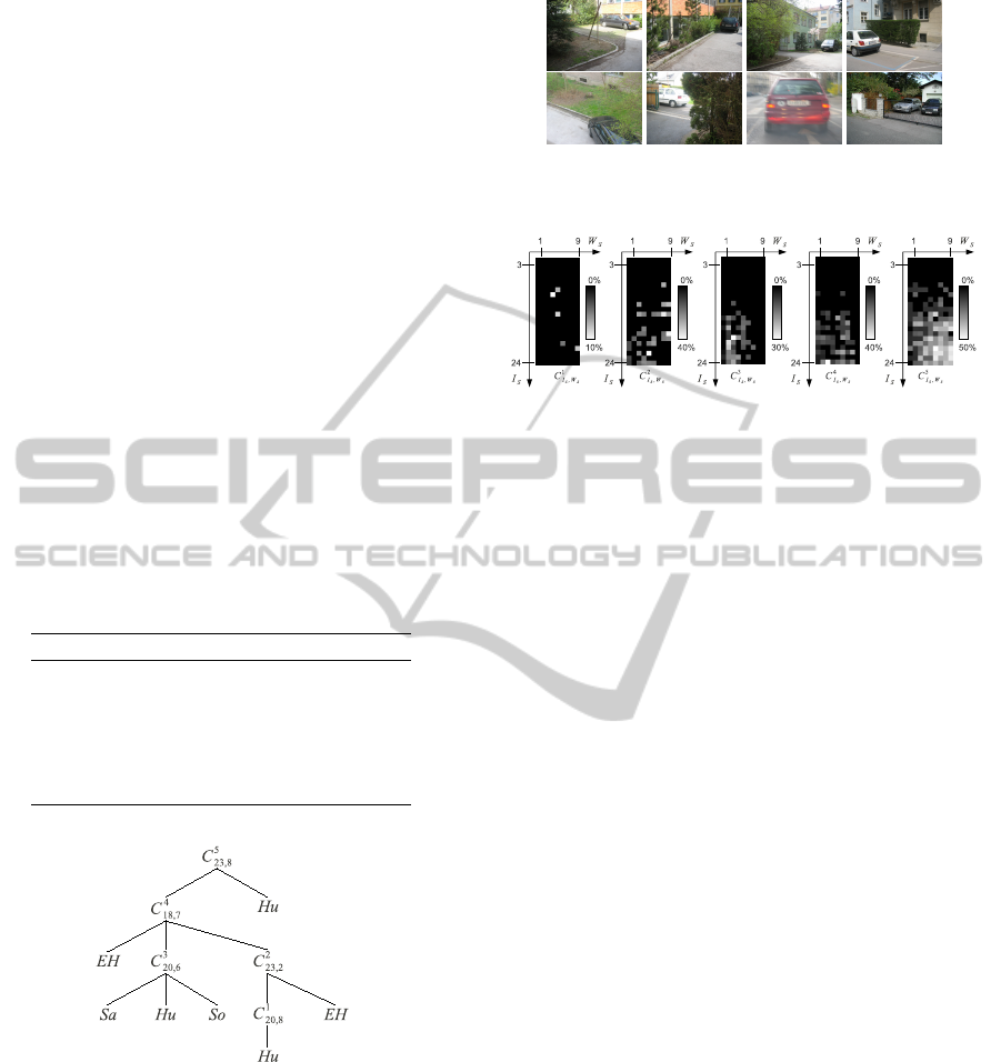
Figure 4: Some examples of images belonging to the dataset

TU-Graz cars.

Figure 5: Each image shows how the F-measure varies in

the parameter space (I

) for each node C

- C

shown in Figure 3. A white pixel represents a F-measure

equals to the maximum value. Each network was trained on

10 images of the training set and the F-measure was com-

puted on the ﬁrst 10 images of the testing set TU-Graz cars.

3.2 Comparisons

In (Everingham et al., 2005) several innovative meth-

ods for object detection were evaluated on a dataset

containing four classes of objects: motorbikes, bi-

cycles, people and cars. The training and test sets

contain objects having substantial variations in terms

of scale, occlusion, and variability within the class.

These aspect of the dataset allow to better assess an

algorithm and to highlight the beneﬁts and drawbacks

of the same algorithm. Another advantage of this

dataset is the possibility to compare an algorithm with

the whole community that used it.

Our algorithm requires the presence of a GT-Mask

for each training image, and not all the four classes

of objects have that information associated with each

training image. For this reason we used only three

classes of objects bicycles, people and cars and for

each class we use only the training image having a

GT-Mask.

The metrics used here are the same as that used

in (Everingham et al., 2005): the PR-curve and the

Average Precision (AP).

The network showed in Figure 6 represents the

structure used in all the three classes of objects. The

structure of the model used in this experiment was

built with the following rule: we build some of the

nodes which receive in input some features and are

conﬁgured with a small I

value, the maps generated

by these nodes are passed in input to other nodes that

increase the I

value, and so on. In this way we can

see a reﬁnement of the segmentation result through

VISAPP 2011 - International Conference on Computer Vision Theory and Applications

134

every level of the tree towards the root node.

From this experiment we found that the main

problem of our algorithm lies in the dataset with large

differences of scale. Then, trying to force in input

only the area containing the object (see some exam-

ples showed in the ﬁrst row of the Figure 7), we note

that the results increase signiﬁcantly (see MNOD-SI

in Table 2). The model so trained and tested was re-

named MNOD-SI.

In this work a detailed analysis on the best features

for this model has not been done. For this experiment

we used a limited set of features that highlight some

information on color and high frequencies present in

the images. In particular, we used the features Sat-

uration (Sa), Hue (Hu), Brightness (Br), Horizontal

Edges (EH), Vertical Edges (EV ) and Histogram of

Gradient (HoG) conﬁgured in different ways. The

parameter s in EH

and EV

is the scale used on the

input image before to compute the feature. The pa-

rameters (s,b) in HoG

s,b

are the scale used on the in-

put image and the block size respectively. The HoG

feature, as in (Dalal and Triggs, 2005), reads the in-

put values from a sliding window of histograms (cell

block). In this work each histogram is composed by

four bins, a cell block is an area of 6 × 6 pixels and

the neural model used, instead of the SVM, is a MLP.

In Table 2 we compare our model with some meth-

ods presented in (Everingham et al., 2005), while in

Figure 8 the trend of the PR-curve using MNOD-SI

is shown for the three classes of objects. The AP

measure on the three classes of problems considered

was computed using the same conﬁguration showed

in Figure 6 and the standard test set called test1 for

each class of objects of the VOC 2005 Dataset 1.

It is obvious that we could obtain better results by

making a thorough search of the parameters and of the

features, as evidenced in the study showed in Figure 5,

but we will deal with this issue in a future work. Start-

ing from the results obtained using the model MNOD-

SI we are working for a new version able to exploiting

the different scales in images of a particular domain.

A very interesting result is the fact that the model has

a similar behavior on different classes of objects.

4 CONCLUSIONS

In this paper we described an object detection algo-

rithm based on a multiple networks system. It is

composed by a set of neural networks aggregated to-

gether to provide a single output result. The model

was tested and the results were presented, highlight-

ing the potentialities of our solution. The proposed

algorithm can be conﬁgured for different classes of

Table 2: Average precision for the object detection problem

applied to the test set called test1 in VOC 2005 Dataset 1.

The comparison results are taken from (Everingham et al.,

2005).

Method Bicycles People Cars

MNOD 0.01 0.02 0.06

MNOD-SI 0.2 0.21 0.42

Boosted-Histogram 037 0.25 0.663

TU-Darmstadt - - 0.489

Edinburg 0.19 0.002 0.00

INRIA-Dalal - 0.01 0.61

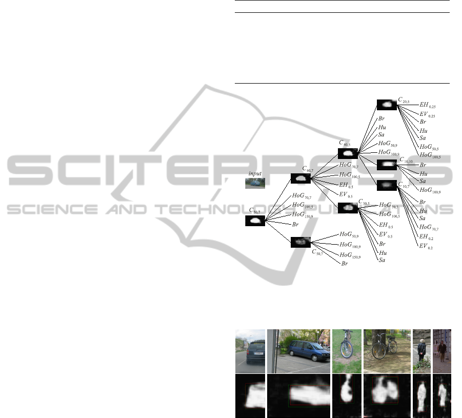
Figure 6: MNOD conﬁguration used for the three categories

of objects in the dataset VOC2005. The model displays the

maps produced by each node C

and the features used in

input, all related to the input image of the testing set.

Figure 7: On the ﬁrst line there are some image examples

of the dataset VOC2005. On the second line the maps pro-

duced by the trained model and the desired bounding box in

green.

object and its nodes may consist of different types

of neural learning strategies. This type of algorithm,

here mainly used for detection, provides an interest-

ing segmentation result that we intend to exploit in

future works.

We obtained good results on many standard

dataset compared to other object detection algorithms.

Moreover, the results show that our algorithm is ro-

bust to the change of perspective for the same object

and at the same time, it is robust for objects of the

LEARNING OBJECT DETECTION USING MULTIPLE NEURAL NETWORKS

135

0.2

0.4

0.6

0.8

0 0.2 0.4 0.6 0.8 1

precision

recall

Precision vs. Recall VOC2005 Dataset 1

cars

people

bicycles

Figure 8: PR curve for the three classes of objects bicycles,

people e cars. The model used for this graph is MNOD-SI.

same type but different forms in different poses or

even articulated and occluded.

The proposed algorithm suffers from some issues

related to datasets with conspicuous differences of

scale for the objects that we want to detect. Therefore

we are working on a different strategy to overcome

this problem. Detection results are dependent on net-

work topology and from the selected set of features.

Then, we are analyzing new search algorithms able to

select the best network conﬁguration.

REFERENCES

Bouchard, G. and Triggs, B. (2005). Hierarchical part-

based visual object categorization. In Proc. CVPR,

pages 710–715.

Crandall, D., Felzenszwalb, P., and Huttenlocher, D. (2005).

Spatial priors for part-based recognition using statisti-

cal models. In Proc. CVPR, pages 10–17.

Csurka, G., Dance, C. R., Fan, L., Willamowski, J., and

Bray, C. (2004). Visual categorization with bags of

keypoints. In In Workshop on Statistical Learning in

Computer Vision, ECCV, pages 1–22.

Dalal, N. and Triggs, B. (2005). Histograms of oriented

gradients for human detection. In Proc. CVPR, pages

886–893.

Everingham, M., Zisserman, A., Williams, C. K. I., Gool,

L. V., Allan, M., Bishop, C. M., Chapelle, O., Dalal,

N., Deselaers, T., Dork, G., Duffner, S., Eichhorn, J.,

Farquhar, J. D. R., Fritz, M., Garcia, C., Grifﬁths, T.,

Jurie, F., Keysers, D., Koskela, M., Laaksonen, J., Lar-

lus, D., Leibe, B., Meng, H., Ney, H., Schiele, B.,

Schmid, C., Seemann, E., Shawe-taylor, J., Storkey,

A., Szedmak, O., Triggs, B., Ulusoy, I., Viitaniemi,

V., and Zhang, J. (2005). The 2005 pascal visual ob-

ject classes challenge. In Selected Proceedings of the

First PASCAL Challenges Workshop.

Fei-fei, L. (2005). A bayesian hierarchical model for learn-

ing natural scene categories. In Proc. CVPR, pages

524–531.

Fergus, R., Perona, P., and Zisserman, A. (2003). Ob-

ject class recognition by unsupervised scale-invariant

learning. In Proc. CVPR, pages 264–271.

Fischler, M. and Elschlager, R. (1973). The representation

and matching of pictorial structures. Computers, IEEE

Transactions on, C-22(1):67 – 92.

Leibe, B. and Schiele, B. (2003). Interleaved object cate-

gorization and segmentation. In Proc. BMVC, pages

759–768.

Riedmiller, M. and Braun, H. (1993). A direct adap-

tive method for faster backpropagation learning: The

rprop algorithm. In IEEE INTERNATIONAL CON-

FERENCE ON NEURAL NETWORKS, pages 586–

591.

Riesenhuber, M. and Poggio, T. (1999). Hierarchical mod-

els of object recognition in cortex. Nature Neuro-

science, 2(11):1019–1025.

Schmid, C. (2006). Beyond bags of features: Spatial

pyramid matching for recognizing natural scene cat-

egories. In Proc. CVPR, pages 2169–2178.

Serre, T., Wolf, L., and Poggio, T. (2005). Object recog-

nition with features inspired by visual cortex. In

Proceedings of the Conference on Computer Vision

and Pattern Recognition, CVPR ’05, pages 994–1000,

Washington, DC, USA. IEEE Computer Society.

Sharkey, A. J. (1999). Combining Artiﬁcial Neural Nets:

Ensemble and Modular Multi-Net Systems, chapter

Multi-Net Systems. Springer.

Todorovic, S. and Ahuja, N. (2006). Extracting subimages

of an unknown category from a set of images. In Proc.

CVPR, pages 927–934.

Utgoff, P. E. (1988). Perceptron trees: A case study in hy-

brid concept representations. In AAAI, pages 601–606.

Zhu, L. and Yuille, A. (2006). A hierarchical compositional

system for rapid object detection. In Proc. NIPS.

VISAPP 2011 - International Conference on Computer Vision Theory and Applications

136