EFFICIENT DYNAMICAL COMPUTATION

OF PRINCIPAL COMPONENTS

Darko Dimitrov

, Mathias Holst

, Christian Knauer

and Klaus Kriegel

Freie Universit

at Berlin, Institute of Computer Science, Takustraße 9, D-14195 Berlin, Germany

{ }

Universit

at Rostock, Institute of Computer Science, Albert Einstein Straße 21, D-18059 Rostock, Germany

Universit

at Bayreuth, Institute of Computer Science, Universit

atsstraße 30, D-95447 Bayreuth, Germany

Keywords:

Principal Component Analysis, Dynamic Computation, Bounding Box Algorithms, Approximation Algo-

rithms.

Abstract:

In this paper we consider the problem of updating principal components of a point set in R

when points

are added or deleted from the point set. A recent result of (P

ebay, 2008) implies an efﬁcient solution for

that problem when points are added to a discrete point set. Here, we extend that result for deletions in the

discrete case, and for both additions and deletions for continuous point sets in R

and R

. In both cases,

discrete and continuous, no additional data structures or storage are needed for computing the new principal

components. An important application of the above results is the dynamical computation of bounding boxes

based on principal component analysis. PCA bounding boxes are very often used in many ﬁelds, among others

in computer graphics, for example, for ray tracing, fast rendering, collision detection, or video compression

algorithms. Since some version of PCA bounding boxes have guaranties on their size (volume), they are also

of interest in applications where the guaranty of the approximation quality is required. We have designed and

implemented algorithms for computing dynamically PCA bounding boxes in R

1 INTRODUCTION

Principal component analysis (PCA) (Jolliffe, 2002)

is probably the oldest and best known of the tech-

niques of multivariate analysis. The central idea and

motivation of PCA is to reduce the dimensionality of a

point set by identifying the most signiﬁcant directions

(principal components). Let P = {~p

,~p

,...,~p

} be a

set of vectors (points) in R

, and~µ = (µ

,µ

,...,µ

) ∈

be the center of gravity of P. For 1 ≤ k ≤ d, we

use p

i,k

to denote the k-th coordinate of the vector p

Given two vectors ~u and ~v, we use h~u,~vi to denote

their inner product. For any unit vector ~v ∈ R

, the

variance of P in direction ~v is

var(P,~v) =

∑

i=1

h~p

−~µ ,~vi

. (1)

The most signiﬁcant direction corresponds to the

unit vector ~v

such that var(P,~v

) is maximum. In

This research was supported by the German Research

Foundation (DFG), grant No. AL 253/6-2, Project “Entwurf

und Analyse anwendungsbezogener geometrischer Algo-

rithmen”.

general, after identifying the j most signiﬁcant di-

rections ~v

,...,~v

, the ( j + 1)-th most signiﬁcant di-

rection corresponds to the unit vector ~v

j+1

such that

var(P,~v

j+1

) is maximum among all unit vectors per-

pendicular to ~v

,~v

,...,~v

It can be veriﬁed that for any unit vector~v ∈ R

var(P,~v) = hΣ~v,~vi, (2)

where Σ is the covariance matrix of P. Σ is a sym-

metric d × d matrix where the (i, j)-th component,

i j

,1 ≤ i, j ≤ d, is deﬁned as

i j

∑

k=1

k,i

−µ

)(p

k, j

−µ

). (3)

The procedure of ﬁnding the most signiﬁcant di-

rections, in the sense mentioned above, can be formu-

lated as an eigenvalue problem. If λ

≥λ

≥··· ≥ λ

are the eigenvalues of Σ, then the unit eigenvector ~v

for λ

is the j-th most signiﬁcant direction. Since the

matrix Σ is symmetric positive semideﬁnite, its eigen-

vectors are orthogonal, all λ

s are non-negative and

= var(P,~v

Dimitrov D., Holst M., Knauer C. and Kriegel K..

EFFICIENT DYNAMICAL COMPUTATION OF PRINCIPAL COMPONENTS.

DOI: 10.5220/0003324800850093

In Proceedings of the International Conference on Computer Graphics Theory and Applications (GRAPP-2011), pages 85-93

ISBN: 978-989-8425-45-4

 2011 SCITEPRESS (Science and Technology Publications, Lda.)

Computation of the covariance matrix can be done

in O(d

n) time, while computation of the eigenval-

ues, when d is not very large, can be done in O(d

)

time, for example with the Jacobi or the QR method

(Press et al., 1995). Thus, the time complexity of

computing principal components of n points in R

O(d

n + d

). The multiplicative factor of O(d

) and

the additive factor of O(d

) throughout the paper will

be omitted, since we will assume that d is ﬁxed. For

very large d, the problem of computing eigenvalues

is non-trivial. In practice, the above mentioned meth-

ods for computing eigenvalues converge rapidly. In

theory, it is unclear how to bound the running time

combinatorially and how to compute the eigenvalues

in decreasing order. In (Cheng and Y. Wang, 2008)

a modiﬁcation of the Power method (Parlett, 1998) is

presented, which can give a guaranteed approxima-

tion of the eigenvalues with high probability.

Examples of applications of PCA include data

compression, exploratory data analysis, visualization,

image processing, pattern and image recognition,

time series prediction, detecting perfect and reﬂec-

tive symmetry, and dimension detection. The thor-

ough overview of PCA’s applications can be found

for example in the textbooks (Duda et al., 2001) and

(Jolliffe, 2002). Most of the applications of PCA are

non-geometric in their nature. However, there are

also few purely geometric applications that are quite

widespread in computer graphics. Example are the

estimation of the undirected normals of the point sets

or computing PCA bounding boxes (bounding boxes

determined by the principal components of the point

set).

Contributions and Organization of the Paper. Dy-

namic versions of the above applications, i.e., when

the point set (population) changes, are of big impor-

tance and interest. Efﬁcient solutions of those prob-

lems depend heavily on an efﬁcient dynamic compu-

tation of the principal components (eigenvectors of

the covarince matrix). Dynamic updates of variances

in different settings have been studied since the six-

ties (Chan et al., 1979), (Knuth, 1998), (P

ebay, 2008),

(Welford, 1962), (West, 1979). Recently, in a techni-

cal report (P

ebay, 2008) also investigated the dynamic

maintenance of covariance matrices. Our contribution

extends these results in the following directions:

1. We also take into account the operation of point

deletions.

2. We study the dynamic computation of principal

components in the continuous version.

3. We combine the dynamic PCA versions with ef-

ﬁcient methods for computing PCA bounding

boxes.

We consider the computation of the dynamic PCA

bounding boxes, since it has very important appli-

cations in many ﬁelds including computer graphics,

where the PCA boxes are used, for example, for ray

tracing, fast rendering, video compression algorithms,

or collision detection. Two distinguished hierarchi-

cal data structures from computer graphics used for

representation of 3D surfaces and for rapid interfer-

ence detection, based on PCA bounding boxes, are

the Boxtree (Barequet et al., 1996) and the OBBTree

(Gottschalk et al., 1996). We would like to stress, that

PCA bounding boxes are also of interest in applica-

tions where the guaranty of the approximation qual-

ity is required, since some version of PCA bounding

boxes have guaranties on their size (Dimitrov et al.,

2009b). Based on the theoretical results in this paper,

we have implemented several algorithms for comput-

ing PCA bounding boxes dynamically.

The organization and the main results of the paper

are as follows: In Section 2 we consider the prob-

lem of updating the principal components of a set of

n points, when m points are added or deleted from

the point set. For both operations performed on a dis-

crete point set in R

, we can compute the new prin-

cipal components in O(m) time for ﬁxed d. This is a

signiﬁcant improvement over the commonly used ap-

proach of recomputing the principal components from

scratch, which takes O(n + m) time. We also consider

the computation of the principal components of a dy-

namic continuous point set. We give closed form so-

lutions when the point set is a convex polytope R

Due to the space limitation, the cases when the point

set is the boundary of a convex polytope in R

or R

or a convex polygon in R

, are left for an extended

version of this paper. In Section 3 we present and

verify the correctness of some theoretical results pre-

sented in the Section 2. We have implemented several

dynamic PCA bounding box algorithms and evaluated

their performances. Conclusion and open problems

are presented in Section 4.

2 UPDATING THE PRINCIPAL

COMPONENTS EFFICIENTLY

2.1 Discrete Case in R

Here, we consider the problem of updating the

covariance matrix Σ of a discrete point set P =

{~p

,~p

,...,~p

} in R

, when m points are added or

deleted from P. The recent result of (P

ebay, 2008)

implies the same solution that we have obtained for

additions. Since the derivation of the closed form so-

GRAPP 2011 - International Conference on Computer Graphics Theory and Applications

lutions for deletions is similar to that for additions,

and due to the space limitation here, we just state the

main result related to the discrete points sets without

proof.

Theorem 2.1 Let P be a set of n points in R

with

known covariance matrix Σ. Let P

be a point set in

, obtained by adding or deleting m points from P.

The principal components of P

can be computed in

O(m) time for ﬁxed d.

The principal components of discrete point sets can

be strongly inﬂuenced by point clusters (Dimitrov

et al., 2009b). To avoid the inﬂuence of the distribu-

tion of the point set, often continuous sets, especially

the convex hull of a point set is considered, which

lead to so-called continuous PCA. Computing PCA

bounding boxes (Gottschalk et al., 1996), (Dimitrov

et al., 2009a), or retrieval of 3D-objects (Vrani

c et al.,

2001), are typical applications where continuous PCA

are of interest.

2.2 Continuous Case in R

Here, we consider the computation of the principal

components of a dynamic continuous point set. We

present a closed form-solutions when the point set is

a convex polytope or the boundary of a convex poly-

tope in R

or R

. When the point set is the boundary

of a convex polytope, we can update the new principal

components in O(k) time, for both deletion and addi-

tion, under the assumption that we know the k facets

in which the polytope changes. Under the same as-

sumption, when the point set is a convex polytope in

or R

, we can update the principal components in

O(k) time after adding points. But, to update the prin-

cipal components after deleting points from a convex

polytope in R

or R

we need O(n) time. This is due

to the fact that, after a deletion the center of gravity of

the old convex hull (polyhedron) could lie outside the

new convex hull, and therefore, a retetrahedralization

is needed (see Subsection 2.2.1).

Due to the space limitation, we present in this sec-

tion only the closed-form solutions for a convex poly-

tope in R

, and leave the cases when the point set is

the boundary of a convex polytope in R

or R

, or a

convex polygon in R

, for an extended version of this

paper.

2.2.1 Continuous PCA over a Convex

Polyhedron in R

Let P be a point set in R

, and let X be its convex

hull. We assume that the boundary of X is triangula-

ted (if it is not, we can triangulate it in a preprocessing

step). We choose an arbitrary point ~o in the interior of

X, for example, we can choose ~o to be the center of

gravity of the boundary of X. Each triangle from the

boundary together with ~o forms a tetrahedron. Let

the number of such formed tetrahedra be n. The k-th

tetrahedron, with vertices ~x

1,k

,~x

2,k

,~x

3,k

,~x

4,k

= ~o, can

be represented in a parametric form by

(s,t,u) =

4,k

+ s(~x

1,i

−~x

4,k

) +t (~x

2,i

−~x

4,k

) +u (~x

3,i

−~x

4,k

), for

0 ≤s,t, u ≤ 1, and s +t + u ≤1. For 1 ≤i ≤3, we use

i, j,k

to denote the i-th coordinate of the vertex ~x

the tetrahedron

The center of gravity of the k-th tetrahedron is

~µ

1−s

1−s−t

ρ(

(s,t,u))

(s,t,u)du dt ds

1−s

1−s−t

ρ(

(s,t,u))du dt ds

where ρ(

(s,t,u)) is a mass density at a point

(s,t,u). Since we can assume ρ(

(s,t,u)) = 1,

we have

~µ

1−s

1−s−t

(s,t,u)du dt ds

1−s

1−s−t

du dt ds

1,k

+~x

2,k

+~x

3,k

+~x

4,k

The contribution of each tetrahedron to the center of

gravity of X is proportional to its volume. If M

is the

3×3 matrix whose l-th row is~x

l,k

−~x

4,k

, for l = 1...3,

then the volume of the k-th tetrahedron is

= volume(Q

) =

|det(M

We introduce a weight to each tetrahedron that is pro-

portional to its volume, deﬁne as

∑

k=1

where v is the volume of X. Then, the center of grav-

ity of X is

~µ =

∑

k=1

~µ

The covariance matrix of the k-th tetrahedron is

1−s

1−s−t

(

(s,t,u)−~µ)(

(s,t,u)−~µ)

du dt ds

1−s

1−s−t

du dt ds



∑

j=1

∑

h=1

(~x

j,k

−~µ)(~x

h,k

−~µ)

∑

j=1

(~x

j,k

−~µ)(~x

j,k

−~µ)



The (i, j)-th element of Σ

, i, j ∈ {1, 2, 3}, is

i j,k



∑

l=1

∑

h=1

i,l,k

−µ

)(x

j,h,k

−µ

∑

l=1

i,l,k

−µ

)(x

j,l,k

−µ

)



with ~µ = (µ

,µ

). Finally, the covariance ma-

trix of X is

Σ =

∑

i=1

EFFICIENT DYNAMICAL COMPUTATION OF PRINCIPAL COMPONENTS

with (i, j)-th element

i j



∑

k=1

∑

l=1

∑

h=1

i,l,k

−µ

)(x

j,h,k

−µ

∑

k=1

∑

l=1

i,l,k

−µ

)(x

j,l,k

−µ

)



We would like to note that the above expressions

hold also for any non-convex polyhedron that can be

tetrahedralized. A star-shaped object, where ~o is the

kernel of the object, is such example.

Adding Points

We add points to P, obtaining a new point set P

. Let

be the convex hull of P

. We consider that X

obtained from X by deleting n

, and adding n

tetra-

hedra. Let

∑

k=1

n+n

∑

k=n+1

−

n+n

∑

k=n+n

= v +

n+n

∑

k=n+1

−

n+n

∑

k=n+n

The weight of a tetrahedron Q

is now

The center of gravity of X

~µ

∑

k=1

~µ

n+n

∑

k=n+1

~µ

−

n+n

∑

k=n+n

~µ

∑

k=1

~µ

n+n

∑

k=n+1

~µ

−

n+n

∑

k=n+n

~µ

v~µ +

n+n

∑

k=n+1

~µ

−

n+n

∑

k=n+n

~µ

(4)

Let

~µ

n+n

∑

k=n+1

~µ

, and ~µ

n+n

∑

k=n+n

~µ

Then, we can rewrite (4) as

~µ

~µ +~µ

−~µ

. (5)

The i-th component of~µ

and~µ

, 1 ≤i ≤3, is denoted

by µ

i,a

and µ

i,d

, respectively. The (i, j)-th component,

i j

, 1 ≤ i, j ≤ 3, of the covariance matrix Σ

of X

i j



∑

k=1

∑

l=1

∑

h=1

i,l,k

−µ

)(x

j,h,k

−µ

∑

k=1

∑

l=1

i,l,k

−µ

)(x

j,l,k

−µ

n+n

∑

k=n+1

∑

l=1

∑

h=1

i,l,k

−µ

)(x

j,h,k

−µ

n+n

∑

k=n+1

∑

l=1

i,l,k

−µ

)(x

j,l,k

−µ

)−

n+n

∑

k=n+n

∑

l=1

∑

h=1

i,l,k

−µ

)(x

j,h,k

−µ

)−

n+n

∑

k=n+n

∑

l=1

i,l,k

−µ

)(x

j,l,k

−µ

)



Let

i j

(σ

i j,11

+ σ

i j,12

+ σ

i j,21

+ σ

i j,22

−σ

i j,31

−σ

i j,32

where

i j,11

∑

k=1

∑

l=1

∑

h=1

i,l,k

−µ

)(x

j,h,k

−µ

), (6)

i j,12

∑

k=1

∑

l=1

i,l,k

−µ

)(x

j,l,k

−µ

), (7)

i j,21

n+n

∑

k=n+1

∑

l=1

∑

h=1

i,l,k

−µ

)(x

j,h,k

−µ

), (8)

i j,22

n+n

∑

k=n+1

∑

l=1

i,l,k

−µ

)(x

j,l,k

−µ

), (9)

i j,31

n+n

∑

k=n+n

∑

l=1

∑

h=1

i,l,k

−µ

)(x

j,h,k

−µ

(10)

i j,32

n+n

∑

k=n+n

∑

l=1

i,l,k

−µ

)(x

j,l,k

−µ

). (11)

GRAPP 2011 - International Conference on Computer Graphics Theory and Applications

Plugging-in the values of µ

and µ

in (6), we obtain:

i j,11

∑

k=1

∑

l=1

∑

h=1

i,l,k

−

−µ

i,a

+ µ

i,d

)·

j,h,k

−

−µ

j,a

+ µ

j,d

)

∑

k=1

∑

l=1

∑

h=1

i,l,k

−µ

+ µ

(1 −

) −µ

i,a

+ µ

i,d

)

j,h,k

−µ

+ µ

(1 −

) −µ

j,a

+ µ

j,d

)

∑

k=1

∑

l=1

∑

h=1

i,l,k

−µ

)(x

j,h,k

−µ

)

∑

k=1

∑

l=1

∑

h=1

i,l,k

−µ

)(µ

(1 −

) −µ

j,a

+ µ

j,d

)

∑

k=1

∑

l=1

∑

h=1

(µ

(1 −

) −µ

i,a

+ µ

i,d

)(x

j,h,k

−µ

)

∑

k=1

∑

l=1

∑

h=1

(µ

(1 −

) −µ

i,a

+ µ

i,d

)·

(µ

(1 −

) −µ

j,a

+ µ

j,d

(12)

Since

∑

k=1

∑

l=1

i,l,k

−µ

) = 0, 1 ≤i ≤3, we have

i j,11

∑

k=1

∑

l=1

∑

h=1

i,l,k

−µ

)(x

j,h,k

−µ

)

∑

k=1

∑

l=1

∑

h=1

(µ

(1 −

) −µ

i,a

+ µ

i,d

)·

(µ

(1 −

) −µ

j,a

+ µ

j,d

)

∑

k=1

∑

l=1

∑

h=1

i,l,k

−µ

)(x

j,h,k

−µ

)

+ 16

(µ

(1 −

) −µ

i,a

+ µ

i,d

)·

(µ

(1 −

) −µ

j,a

+ µ

j,d

(13)

Plugging-in the values of µ

and µ

in (7), we obtain:

i j,12

∑

k=1

∑

l=1

i,l,k

−

−µ

i,a

+ µ

i,d

)·

j,h,k

−

−µ

j,a

+ µ

j,d

)

∑

k=1

∑

l=1

i,l,k

−µ

+ µ

(1 −

) −µ

i,a

+ µ

i,d

)·

j,h,k

−µ

+ µ

(1 −

) −µ

j,a

+ µ

j,d

)

∑

k=1

∑

l=1

i,l,k

−µ

)(x

j,h,k

−µ

)

∑

k=1

∑

l=1

i,l,k

−µ

)(µ

(1 −

) −µ

j,a

+ µ

j,d

)

∑

k=1

∑

l=1

(µ

(1 −

) −µ

i,a

+ µ

i,d

)(x

j,h,k

−µ

)

∑

k=1

∑

l=1

(µ

(1 −

) −µ

i,a

+ µ

i,d

)·

(µ

(1 −

) −µ

j,a

+ µ

j,d

(14)

Since

∑

k=1

∑

l=1

i,l,k

−µ

) = 0, 1 ≤i ≤3, we have

i j,12

∑

k=1

∑

l=1

i,l,k

−µ

)(x

j,h,k

−µ

)

∑

k=1

∑

l=1

(µ

(1 −

) −µ

i,a

+ µ

i,d

)·

(µ

(1 −

) −µ

j,a

+ µ

j,d

)

∑

k=1

∑

l=1

i,l,k

−µ

)(x

j,h,k

−µ

)

+ 4

(µ

(1 −

) −µ

i,a

+ µ

i,d

)·

(µ

(1 −

) −µ

j,a

+ µ

j,d

(15)

From (14) and (15), we obtain

i j,1

= σ

i j,11

+ σ

i j,12

= σ

i j

+ 20

(µ

(1 −

) −µ

i,a

+ µ

i,d

)·

(µ

(1 −

) −µ

j,a

+ µ

j,d

(16)

Note that σ

i j,1

can be computed in O(1) time. The

components σ

i j,21

and σ

i j,22

can be computed in

O(n

) time, while O(n

) time is needed to compute

i j,31

and σ

i j,32

. Thus,

and

i j

(σ

i j,11

+ σ

i j,12

+ σ

i j,21

+ σ

i j,22

+ σ

i j,31

+ σ

i j,32

)

(σ

i j

+ σ

i j,21

+ σ

i j,22

+ σ

i j,31

+ σ

i j,32

)

(µ

(1 −

) −µ

i,a

+ µ

i,d

)(µ

(1 −

) −µ

j,a

+ µ

j,d

)

(17)

can be computed in O(n

+ n

) time.

EFFICIENT DYNAMICAL COMPUTATION OF PRINCIPAL COMPONENTS

Deleting Points

Let the new convex hull be obtained by deleting n

tetrahedra from and adding n

tetrahedra to the old

convex hull. If the interior point ~o (needed for a

tetrahedronization of a convex polytope), after sev-

eral deletions, lies inside the new convex hull, then

the same formulas and time complexity, as by adding

points, follow. If ~o lie outside the new convex hull,

then, we need to choose a new interior point~o

, and re-

compute the new tetrahedra associated with it. Thus,

we need in total O(n) time to update the principal

components.

3 PRACTICAL VARIANTS OF

DYNAMICAL PCA BOUNDING

BOXES AND EXPERIMENTAL

RESULTS

The main focus in this section is to show the advan-

tages of the theoretical results presented in this pa-

per in the context of computing dynamic PCA bound-

ing boxes. We present three practical simple algo-

rithms, and compare their performances. The algo-

rithms were implemented in C#, C++ and OpenGL,

and tested on a Core Duo 2.33GHz with 2GB mem-

ory. All algorithms use the result mentioned in Sec-

tion 2.1 to compute the principal components. They

differ only in how the extremal points along the prin-

cipal components are found. The implemented algo-

rithms are the following:

• PCA-AP (PCA-all-points) - ﬁnds the extremal

points by going through all points.

• PCA-AGP (PCA-all-grid-points) - the space is

discretized by a regular three dimensional axis-

aligned grid, with cells of size ε ×ε ×ε. See Fig-

ure 1 for an illustration. The grid size is chosen

relatively to the size of the object. Each object

is scaled such that its diameter is 1. The val-

ues of ε are between 0.001 and 1. The corners

of non-empty cells are candidates for extremal

points along the principal directions.

• PCA-EGP (PCA-extremal-grid-points) - this is

an improvement of the PCA-AGP algorithm. To

each vertical grid line, i.e., orthogonal to the XY

plane, two extremal corners of the non-empty cell

are computed. Thus, we reduced the number

of candidates for extremal points from O(

) to

We further reduce the number of points consid-

ered in the PCA-AGP and PCA-EGP algorithms by

replacing the cell corners with the centers of gravity

of the cells. Afterwords, we expand the resulting box

√

3ε/2 to ensure that the box contains all origi-

nal points. We have implemented also these variants,

but, since for a reasonable big grid size (ε ≥ 0.01) the

running time improvements are negligible, we report

here only the results of the base variants of the algo-

rithms PCA-AGP and PCA-EGP. For very dense grid

the improved version of the both algorithms give bet-

ter results.

In the following experiments, we add (delete) ran-

dom points from the point set, and compare the re-

sults of a dynamical versions of PCA bounding boxes

with their corresponding static versions (when the co-

variance matrix of the point set is computed from

scratch). The time of computing, the volume of a

bounding box, and the grid density are parameters of

interest in this evaluation study. The tests were per-

formed on a large number of real graphics models

taken from various publicly available sources (Stan-

ford 3D scanning repository, 3D Cafe). Typical sam-

ples of the results are given in Table 1, Table 2, and

Table 3.

The main conclusions of the experiments are as fol-

lows:

• As expected from the theoretical results, the dy-

namic versions of the algorithms are signiﬁcantly

faster than their static counterparts. Typically, the

dynamic versions are about an order of magnitude

faster (see Table 1).

• The dynamic PCA-AP algorithm is not only sig-

niﬁcantly faster than its static version, it is also

faster than the static version of the PCA-AGP and

PCA-EGP algorithms. This is due to the fact that

the brute force manner of ﬁnding the extremal

points is faster than computing the covariance ma-

trix of the new point set from scratch, although

both algorithms require O(n) time in the asymp-

totic analysis.

• Clearly, the PCA-AGP and PCA-EGP algorithms,

that exploit the grid subdivision structure, are

faster than the PCA-AP algorithm. The price that

must be paid for this is twofold. First, an extra

preprocessing time for building the grid is needed.

For the example considered in Table 1, computing

the grid takes about 0.4 seconds for the PCA-AGP

algorithm, and about 0.43 for the PCA-EGP algo-

rithm. Second, the resulting bounding boxes are

less precise (see Table 2).

• As it is shown in Table 3, for grids that are not

very sparse (ε ≤ 0.03), the approximated PCA

bounding boxes computed by the PCA-AGP and

PCA-EGP algorithms are quite close to the exact

PCA bounding boxes.

GRAPP 2011 - International Conference on Computer Graphics Theory and Applications

(a)

(b)

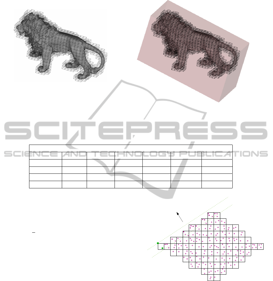
Figure 1: (a) A real world object and its corresponding grid for ε = 0.03. Only the non-empty cells are visualized. (b) The

bounding box of the object obtained by the PCA-AGP algorithm.

Table 1: Time needed by the PCA bounding box algorithms for the lion model (183408 points). The values in the table are

the average of results of 100 runs of the algorithms, each time adding/deleting the corresponding number of points.

Adding/deleting points, ε = 0.005

1pnt 1pnt 100 pnts 100 pnts 1000 pnts 1000 pnts

algorithm static dynamic static dynamic static dynamic

PCA-AP 0.166 s 0.014 s 0.171 s 0.015 s 0.172 s 0.016 s

PCA-AGP 0.092 s 0.010 s 0.093 s 0.009 s 0.990 s 0.017 s

PCA-EGP 0.081 s 0.006 s 0.082 s 0.006 s 0.092 s 0.014 s

Tighter bounding boxes for the PCA-AGP and PCA-

EGP algorithms can be obtained by the following ap-

proach. Let P

be the supporting plane at the extremal

grid point along one principal direction, and let P

the plane parallel to P

, such that the distance between

and P

√

3ε/2, and P

intersect or is tangent to

the grid. We denote by S the subspace between P

and P

. Then, the candidates points for the chosen

principal direction, that determine the tight bounding

box, are all original points that belong to cells that

have intersection with S. See Fig. 2 for an illustration.

However, in the worst case all original points have to

be checked.

Further (theoretical) improvement of the algo-

rithms presented here could be obtained if, instead of

the point set, we consider its convex hull when we

look for extremal points. This only makes sense if

the convex hull is computed dynamically. Otherwise,

computing the static convex hull of the points will be

more expensive than ﬁnding the exact extremal points

by scanning all points.

P C

Figure 2: For the principal direction PC

, the algorithms

PCA-AGP and PCA-EGP detect the point g

as extremal

grid point, and the point x as extremal point of the original

point set. However, there are other points (the violet colored

circles) that are further than x along PC

3.1 Computing efﬁciently a Bounding

Box of Several Objects

An interesting application of the closed-form solu-

tions from Section 2 is to compute the principal com-

ponents of two or more objects with already known

covariance matrices. Thus, for ﬁxed d the new co-

variance matrix Σ and the new principal components

EFFICIENT DYNAMICAL COMPUTATION OF PRINCIPAL COMPONENTS

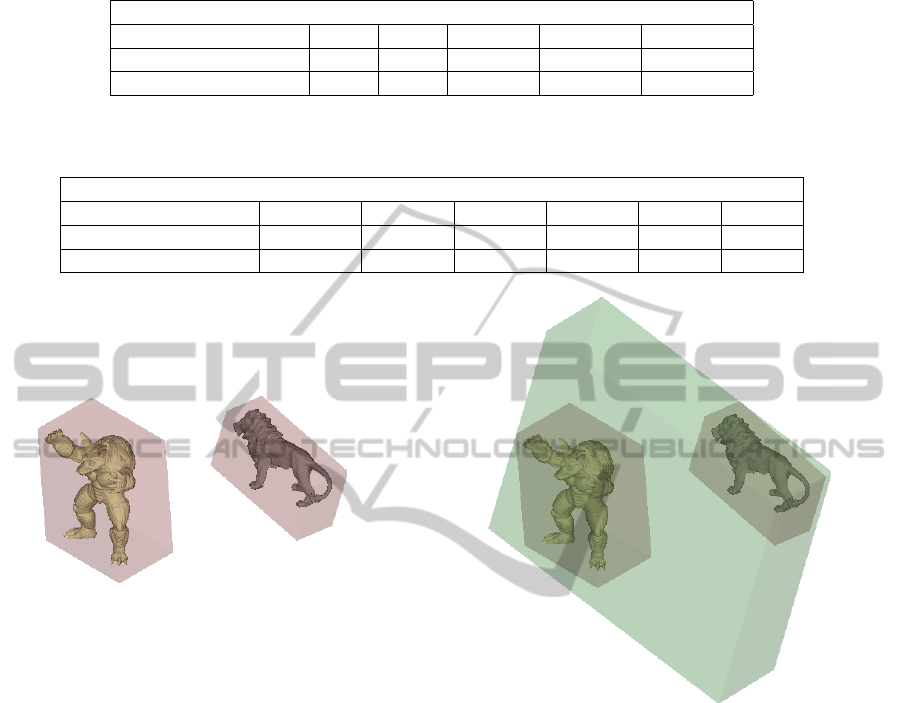
Table 2: Volume of the PCA bounding box algorithms for the lion model. The values in the table are the average of results of

100 runs of the algorithms, each time adding the corresponding number of points.

Adding points, dynamic version, ε = 0.005

algorithm 1pnt 10pnt 100 pnts 1000 pnts 10000 pnts

PCA-AP 285.5 644.6 856.3 1149.1 1236.4

PCA-AGP, PCA-EGP 295.5 662.7 880.3 1221.8 1263.2

Table 3: Volumes of the PCA bounding boxes algorithms for lion model for different grid density. The values in the table are

the average of results of 100 runs of the algorithms, each time adding the corresponding number of points.

Adding 100 points, dynamic version

algorithm ε = 0.005 ε = 0.01 ε = 0.03 ε = 0.05 ε = 0.1 ε = 0.2

PCA-AP 856.3 856.3 856.3 856.3 856.3 856.3

PCA-AGP, PCA-EGP 880.3 904.3 942.3 1080.1 1292.7 2324.8

(b)(a)

Figure 3: (a) Two objects with their PCA bounding boxes. (b) The common PCA bounding box. Computing the common

PCA bounding box dynamically takes 0.004 seconds, while the static version takes 0.02 seconds.

can be computed also in O(1) time.

This is a signiﬁcant improvement over the com-

monly used approach of computing the principal com-

ponents from scratch, which takes time linear in the

number of points. Efﬁcient computation of the com-

mon PCA bounding box of several objects is straight-

forward. See Fig. 3 for an illustration in R

4 CONCLUSIONS AND FUTURE

WORK

The main contributions of this paper are the closed-

form solutions for updating the principal components

of a dynamic point set. The advantages of the theo-

retical results were veriﬁed and presented in the con-

text of computing dynamic PCA bounding boxes, a

very important application in many ﬁelds including

computer graphics, where the PCA boxes are used to

maintain hierarchical data structures for fast render-

ing of a scene or for collision detection. We have pre-

sented three practical simple algorithms and compare

their performances.

An interesting open problem is to ﬁnd a closed-

form solution for dynamical point sets different from

convex polyhedra, for example, implicit surfaces or

B-splines. An implementation of computing princi-

pal components in a dynamic and continuous setting

is planned for future work. Applications of the results

presented here in other ﬁelds, like computer vision or

visualization, are of high interest.

There are several further improvements and open

problems regarding computing dynamic PCA bound-

GRAPP 2011 - International Conference on Computer Graphics Theory and Applications

ing boxes. Instead of subdividing the space by a sim-

ple regular grid, one can use more sophisticated data

structures, like octrees or binary space partition-trees

to speed up the time needed to ﬁnd the extremal points

along the principal directions. A practical, imple-

mentable algorithm for computing the dynamic con-

vex hull of the point set (computing extremal points

dynamically) would also improve the dynamic PCA

bounding box algorithms. Finding coresets for dy-

namic PCA bounding boxes will lead to efﬁcient ap-

proximation algorithms for PCA bounding boxes. We

are also not aware of data structures for efﬁcient com-

putation of extremal points both approximately and

dynamically. Such data structures are also of interest.

ACKNOWLEDGEMENTS

The authors would like to thank the anonymous re-

viewers for their helpful comments and suggestions

that improved the quality of the paper.

REFERENCES

Barequet, G., Chazelle, B., Guibas, L. J., Mitchell, J. S. B.,

and Tal, A. (1996). Boxtree: A hierarchical represen-

tation for surfaces in 3D. Computer Graphics Forum,

15:387–396.

Chan, T. F., Golub, G. H., and LeVeque, R. J. (1979). Up-

dating formulae and a pairwise algorithm for comput-

ing sample variances. Technical Report STAN-CS-

79-773, Department of Computer Science, Stanford

University.

Cheng, S.-W. and Y. Wang, Z. W. (2008). Provable di-

mension detection using principal component analy-

sis. Int. J. Comput. Geometry Appl., 18:415–440.

Dimitrov, D., Holst, M., Knauer, C., and Kriegel, K.

(2009a). Closed-form solutions for continuous PCA

and bounding box algorithms. A. Ranchordas et al.

(Eds.): VISIGRAPP 2008, CCIS, Springer, 24:26–40.

Dimitrov, D., Knauer, C., Kriegel, K., and Rote, G. (2009b).

Bounds on the quality of the PCA bounding boxes.

Computational Geometry, 42:772–789.

Duda, R., Hart, P., and Stork, D. (2001). Pattern classiﬁca-

tion. John Wiley & Sons, Inc., 2nd ed.

Gottschalk, S., Lin, M. C., and Manocha, D. (1996). OBB-

Tree: A hierarchical structure for rapid interference

detection. Computer Graphics, 30:171–180.

Jolliffe, I. (2002). Principal Component Analysis. Springer-

Verlag, New York, 2nd ed.

Knuth, D. E. (1998). The art of computer program-

ming, volume 2: seminumerical algorithms. Addison-

Wesley, Boston, 3rd ed.

Parlett, B. N. (1998). The symmetric eigenvalue prob-

lem. Society of Industrial and Applied Mathematics

(SIAM), Philadelphia, PA.

ebay, P. P. (2008). Formulas for robust, one-pass parallel

computation of covariances and arbitrary-order statis-

tical moments. Technical Report SAND2008-6212,

Sandia National Laboratories.

Press, W. H., Teukolsky, S. A., Veterling, W. T., and Flan-

nery, B. P. (1995). Numerical recipes in C: the art

of scientiﬁc computing. Cambridge University Press,

New York, USA, 2nd ed.

Vrani

c, D. V., Saupe, D., and Richter, J. (2001). Tools for

3D-object retrieval: Karhunen-Loeve transform and

spherical harmonics. In IEEE 2001 Workshop Mul-

timedia Signal Processing, pages 293–298.

Welford, B. P. (1962). Note on a method for calculating cor-

rected sums of squares and products. Technometrics,

4:419–420.

West, D. H. D. (1979). Updating mean and variance esti-

mates: an improved method. Communications of the

ACM, 22:532–535.

EFFICIENT DYNAMICAL COMPUTATION OF PRINCIPAL COMPONENTS