
A RAY TRACING BASED MODEL FOR 3D LADAR SYSTEMS
Tomas Chevalier
Division of Information systems, Swedish Defence Research Agency, FOI, Box 1165, 581 11 Linköping, Sweden
Keywords: 3D ladar, Laser radar, Sensor model, Ray tracing, BRDF, Atmosphere.
Abstract: This paper describes an approach to simulate long range laser based 3D imaging sensor systems. The model
is based on a ray tracing principle where a large amount of rays are sent from a sensor towards the scene.
The scene, the target surface, and the atmosphere affect the rays and the final light energy distribution is ac-
quired by a receiver, where sensor data is generated. The approach includes advanced descriptions of the
materials in the scene, and modeling of several effects in the atmosphere and the receiver electronics. A tur-
bulence model is included to achieve realistic long range simulations. Examples of simulations and corre-
sponding real world data collection are shown. Model validations are presented.
1 INTRODUCTION
During the last decade many sensors for 3D data
registration has emerged on the commercial market.
To determine optimal parameters for those sensors a
number of sensor system models have been devel-
oped along with these systems. At FOI (the Swedish
Defence Research Agency) the capability to model
various 3D ladar systems has been developed. A 3D
ladar (sometimes also called 3D laser radar) system
illuminates the scene with a laser and by scanning or
using a matrix detector it collects a 3D geometry
description of the scene, usually together with the
intensity response. Related works show some ap-
proaches and examples of modeling tools, but either
some important parts are ignored, as the atmosphere
simulations, or the models are too simplified.
The first step of simulation was focused on cor-
rectly retrieving the 3D geometry description, while
further efforts advanced the model to consider many
other aspects. Such aspects include the atmospheric
scintillations, the variation in the reflectance of sepa-
rate scene parts, the complete waveform generation,
and the capability to model several different sensor
system types for registering 3D data. The model
described in this paper is developed for monostatic
systems, where the transmitter and the receiver are
placed on the same platform. This is a common de-
sign for 3D ladar systems. It is mainly implemented
in Matlab, with some computationally heavy parts in
Java and C++.
This paper describes the model developed at FOI
and the physical-based framework that we use in our
development. Section 2 describes the different avail-
able sensor system types that have been considered
for modeling. Section 3 covers the model framework
and theories, especially for the atmosphere propaga-
tion of the laser beam. Details on validation efforts
are given in Section 4. Simulation examples follow
in Section 5 and we conclude the paper in Section 6.
1.1 Related Work
At the beginning of the sensor simulation history
some passive sensor models were effectively im-
plemented into graphics software and even in hard-
ware (Phong, 1975). The simulated sensors were
virtual cameras, and the algorithms were based on
fairly basic ray tracing methods.
These algorithms were developed into more
physically correctness and to include more advanced
sensors (Powell, 2000), who simulates FLIR sensors
and ladar sensors using graphics software.
To make the simulations more realistic and phys-
ically correct, more customized surface reflections
were required. Already in 1967 studies on the reflec-
tions from rough surfaces had been performed (Tor-
rance, 1967), and partly based on this, a physical
reflection model was developed in 1991 (He, 1991).
Some implications of non-Lambertian reflections for
machine vision was published in 1995 (Oren, 1995).
A large number of sensor modeling projects have
been published during the years and during the last
39
Chevalier T..
A RAY TRACING BASED MODEL FOR 3D LADAR SYSTEMS.
DOI: 10.5220/0003322700390048
In Proceedings of the International Conference on Computer Graphics Theory and Applications (GRAPP-2011), pages 39-48
ISBN: 978-989-8425-45-4
Copyright
c
2011 SCITEPRESS (Science and Technology Publications, Lda.)

decade a number of 3D laser sensor models have
evolved. For instance the work behind a 3D imaging
laser scanner model was published in 2005 (Ortiz,
2005) and in 2006 BAE systems published their
work (Grasso, 2006) on a 3D imaging ladar sensor
model.
An American initiative to develop a sensor simu-
lation environment, called Irma, was started by the
Munitions Directorate at AFRL in 1980. At the be-
ginning the purpose was primarily passive IR (infra-
red) simulations, but now the program also includes
radar and ladar simulation capabilities. A number of
publications are showing this progress, for instance
(Savage, 2006; Savage, 2007; Savage, 2008), where
especially (Savage, 2006; Savage, 2007) covers the
ladar sensor development.
In parallel, DSTL began the development of a
simulation program, CameoSim (CAMouflage Elec-
tro-Optic SIMulation) (Moorhead, 2001), to primari-
ly simulate passive electro-optical sensors. This si-
mulation program is commercially available, but
unfortunately, the ladar module (which was sche-
duled to be working a couple of years ago) seems to
be postponed. Sources indicated further progress of
their burst illumination (BIL) simulation, and in
April 2008 they presented 3D imaging sensor simu-
lation based on CameoSim (Harvey, 2008).
A similar approach to the methods presented in
this report was performed by the Center for Ad-
vanced Imaging Ladar (CAIL), at the Utah State
University. Their ladar seeker model, LadarSim
(Budge, 2006), is also based on discrete ray tracing
as the approach presented in this paper, but differs in
some ways. As example they do not consider the
atmosphere, which is a major issue for Ladar system
performance, and their sub resolution pattern inside
each laser pulse is a hexagonal grid instead of the
common quadratic grid. LadarSim is not commer-
cially available and therefore not possible to com-
pare in detail to the model described in this paper.
There are also non-imaging simulation efforts
(Espinola, 2007; Grönwall, 2007), where the aim is
to assist in the sensor performance assessment,
without the need of sensor images.
2 3D LADAR SYSTEMS
Laser based 3D imaging systems can be of many
types, of which some are described in this section.
The most basic Time-of-Flight Laser Scanner that
sends out separate laser pulses and measure the time
to the returning echoes, the Burst Illumination Ladar
which camera controls the high-speed shutter syn-
chronized to the laser pulse to generate range slice
images, and finally the 3D Flash Ladar, which con-
tain a range sensing matrix detector to acquire com-
plete 3D data using only one single laser pulse.
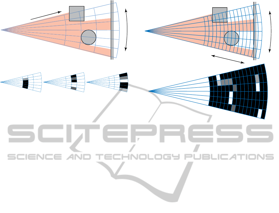
2.1 Time-of-Flight Laser Scanner
The classic version of a 3D imaging laser system is
the Time-of-Flight (TOF) laser scanner, which
works as a range sensing single element detector
mechanically scanned over the scene to collect a
number of laser echoes, as in Figure 1. The direction
and range of each measurement is acquired, and by
using a common coordinate system for all echoes,
the data is registered together. Advanced versions of
this sensor system type allow the complete returning
waveforms to be acquired.
R
a
n
g
e
r
e
s
o
l
u
t
i
o
n
S
p
a
t
i
a
l
r
e
s
o
l
u
t
i
o
n
Figure 1: One-dimensional Time-of-Flight laser scanner
illustration. The sensor system to the left edge is illuminat-
ing the scene to the right (each line is one pulse), where
echoes are registered for each pulse, shown by circles and
crosses. Crosses illustrate multiple echoes from one pulse.
2.2 Burst Illumination Ladar
The Burst Illumination Ladar, also called Gated
Viewing system (Steinvall, 1999), consists of a short
pulsed laser, a high-speed shutter, and a camera.
This system uses an adjustable delay between the
transmitted laser pulse and the high-speed shutter,
while flooding the scene completely with a pulsed
laser. The adjustable delay is used for temporal
scanning, making it possible to register different
range “slices” (or range gates) of the scene, which
means to register light energy that is reflected to-
wards the sensor from a certain distance, see Figure
2. Due to the possibility to use standard cameras,
this sensor system type can have a very dense spatial
resolution, high frame rate, or prf (pulse repetition
frequency).
This sensor data needs post-processing to give
range values in each pixel. This processing is based
on stepping through a number of range slices and
detecting peaks for each pixel. If interpolation is
GRAPP 2011 - International Conference on Computer Graphics Theory and Applications
40
R
a
n
g
e
S
l
i
c
e
1
S
l
i
c
e
2
S
l
i
c
e
3
S
p
a
t
i
a
l
r
e
s
o
l
u
t
i
o
n
Fi r st p u l se
Second pulse
T
hird pulse
Figure 2: One-dimensional Burst Illumination Ladar sys-
tem illustration. The left edge of the top image shows the
sensor system flood illuminating the scene to the right,
where the spatial resolution is set by the camera. The
range dimension is binned by adjusting the delay between
the emitted pulse and the shutter in the detector. One emit-
ted pulse results in one registered slice, as shown in each
of the bottom figures. The gray scale color in the rectan-
gles illustrates the intensity in the echo, where white is
high intensity, and black is low intensity.
performed the depth resolution can be a lot better
than the distance between the slices (Andersson,
2006).
2.3 3D Flash Ladar
The 3D Flash Ladar system collects range data in a
detector element matrix at a reasonable good frame
rate. This makes it possible to register changes in a
scene in three dimensions. Some systems only
record range images while others record a complete
waveform in each pixel, currently at the cost of low
spatial resolution due to large sensor pixel elements.
Figure 3 shows how this sensor system type records
data.
This sensor system type is very interesting for fu-
ture applications, especially since the data is format-
ted as range images and common straight-forward
signal processing methods, like morphological oper-
ations, are applicable directly on the 3D data.
3 SENSOR DATA MODELING
All 3D ladar systems mentioned in Section 2 can be
modelled using the same theory and framework al-
though several parameters differ. This section de-
scribes the framework and main parts of the theory.
R
a
n
g
e
r
e
s
o
l
u
t
i
o
n
S
p
a
t
i
a
l
r
e
s
o
l
u
t
i
o
n
Figure 3: Two-dimensional 3D Flash Ladar system illu-
stration. The scene to the right is flood illuminated from
the left. The spatial resolution is set according to the de-
tector matrix. The range dimension is binned inside the
advanced detector elements, as shown in the bottom fig-
ure, where only one laser pulse is used to generate all the
data. The gray scale color in the rectangles illustrates the
intensity in the echo, where white is high intensity, and
black is low intensity.
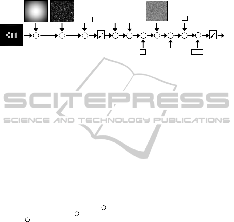
3.1 Model Framework
The model framework is built on four separated sec-
tions of settings; the scene, the laser source, the at-
mosphere, and the receiver.
° The scene settings define the geometry of all the
objects in the scene, i.e. the physical environ-
ment that the sensor system will look at. It
should also contain links to material descriptions,
to allow advanced reflections according to meas-
ured material samples.
° The laser source settings define the way the
scene is illuminated; both temporally and spa-
tially.
° The atmosphere settings define the atmospheric
conditions such as the turbulence strength and
the aerial attenuation, see Section 3.4.
° The receiver settings define the receiver in the
modelled system, together with its optics. The
receiver spatial resolution sets the base resolution
used throughout the simulation. This is multi-
plied by a sub resolution, determining the ability
to image small details in the scene.
Each sub element is represented by a ray sent-
through the optics towards the scene. The propaga
A RAY TRACING BASED MODEL FOR 3D LADAR SYSTEMS
41
×
Target
speckles
*
MTF
opt
Quant
η
Q
×
+
I
dc
*
MTF
speckle
G
×
+
RON
A/D
× ×
Laser energy
distribution
Turbulence
scintillations
Scene /
Target
*
MTF
turb
Figure 4: The model framework. One example scene (a reference board used for the validation measurements) is illumi-
nated by a laser source, turbulence scintillations are multiplied and turbulence blurring effects are applied by convolution.
The right of the ‘Quant’-step contains the target speckle, the optics and the receiver effects. The contributions in this paper
are mainly on the atmospheric simulations, and the quick but accurate combination with MTFs to simulate several types of
signal disturbances.
tion of each ray is calculated in detail to detect inter-
sections in the scene. Each of these intersections
gives the information on which material is hit and in
which angles the light incidents and reflects. To-
gether with the laser spatial energy distribution, and
the atmospheric scintillation, this information is used
to determine the proportion of the transmitted light
that finally hits the sensor element surface. The
simulation framework is described in Figure 4,
where the scene is illuminated by a laser source and
affected by turbulence scintillations and blurring
effects (MTF
turb
). Further on, the signal energy is
quantized into photons (Quant) and blurred even
more by the receiver optics (MTF
opt
). The receiver
electronics defines the quantum efficiency (η
Q
), the
dark current noise (I
dc
), the Gain (G), and the read-
out-noise (RON). In the sensor we also see the target
speckle effects together with blurring (MTF
speckle
).
Finally the signal is converted into a digitally re-
corded data by an A/D-conversion. In the figure,
means element-wise multiplication, means con-
volution, and means element-wise addition.
This figure only shows the spatial part of the en-
ergies, even though the temporal parts are well con-
sidered in all these model steps. The temporal parts
are introduced by considering the scene as an im-
pulse response to the three-dimensional energy dis-
tribution of the laser illumination.
The model parts containing the main contribu-
tions of this paper; the material description, the at-
mosphere modeling, and the sensor data degrada-
tion, are described in the following subsections, to-
gether with a fundamental system transfer function
called the laser radar equation.
3.2 Laser Radar Equation
The one most fundamental relation these simulations
are based upon is the laser radar equation (Jelalian,
1992), that describes the relation between the trans-
mitted and the receiver energy as
2
2
2
aer
R
a
r T syst
r
PP e
R
σ
π
ηρ
−
⎛⎞
=⋅ ⋅⋅ ⋅
⎜⎟
⎝⎠
(3-1)
It is derived from the well known radar equation
(Skolnik, 2008), and identification of the three parts
(to the right of P
T
) in the equation tells us that the
efficiency factor,
η
syst
, is the system efficiency. This
is followed by the (parenthesized) BRDF, see Sec-
tion 3.3, which consists of two factors; first the
BRDF [sr
-1
],
ρ
, and then the solid angle [sr] the re-
ceiver optics aperture covers as seen from the target
reflecting the beam. The last factor, e
-2
σ
R
, is the two-
way aerial transmission due to aerosol particles in
the atmosphere. The laser radar equation is used to
attenuate each ray that passes through the atmos-
phere.
3.3 Material Reflections
To describe the surface reflection properties in detail
the BRDF (bi-directional reflection density func-
tion),
ρ
, is used. The BRDF describes how an inci-
dent beam spreads into different angles. Figure 5
shows a BRDF example, where the amplitude is the
portion of the energy that is reflected (per steradian)
into a specific angle when a light source illuminates
the surface from the direction parallel to the surface
normal. The full BRDF descriptor allows a three-
dimensional reflection distribution, but in our work
we simplify it by using a two-dimensional approxi-
+
*
×
GRAPP 2011 - International Conference on Computer Graphics Theory and Applications
42

mation as in Figure 5, since we model a monostatic
system. Also note that a specific BRDF is valid only
for one wavelength.
-50 0 50
0
0.1
0.2
0.3
0.4
0.5
0.6
0.7
0.8
Angle of incidence [deg]
BRDF [sr
-
1]
A=0.3
B=0.4
m=0.5
s=0.3
Figure 5: A synthetic BRDF example with the amplitude
as a function of the reflected angle when the angle of inci-
dence is parallel to the surface normal. Both a smooth and
a noisy version are shown.
Even though BRDF measurements for several
materials are available, we also need to model the
BRDF analytically, to approximate the reflection
properties for some materials. With some standard
assumptions the BRDF definition (Steinvall, 1997)
follows
cos cos
ss
ss
isis
dP P
dSurface Radiance
Surface Irradiance P P
ρ
θ
θ
ΩΩ
==≈
,
(3-2)
where the variables are depicted in Figure 6. The
reflected solid angle is given by
Ω
s
. The incident and
scattered light flux are represented by P
i
and P
s
. Fi-
nally, the angles of incidence and scattering are
represented by
θ
i
and
θ
s
, respectively. In the monos-
tatic system case, the angle of incidence coincides
with the angle of the relevant scattering light, which
gives us
θ
=
θ
s
=
θ
i
.
There are advanced models to estimate the
BRDF, which relate it to roughness, surface slope,
correlation lengths, refractive index etc., but many
of them tend to get unnecessary complicated. Some
interesting simplified models have been published,
and one of them, a one-dimensional version for mo-
nostatic systems, (Steinvall, 2000) is given by
()
()
()
θ
θ
ρρρ
θ
m
s
diffspec
Be
A
cos
cos
2
2
tan
6
+=+=
−
(3-3)
A and B are constants describing the relation be-
tween the specular and diffuse reflection. Specul
reflection is the strong reflection where
θ
s
=
θ
i
and
Y
X
Z
P
s
P
i
dΩ
s
θ
s
θ
i
φ
s
φ
i
dP
s
Figure 6: Description of the variables used in the BRDF
definition. P shows the light flux while θ/φ are angles. The
subscript s means scattering/emitting and i means incident.
Ω
s
is the solid angle. The figure is adapted from Steinvall
(Steinvall, 2000).
φ
s
=-
φ
i
. It can be recognized as the peak in the middle
of Figure 5. The diffuse reflection supports the base
reflection below the peak in the middle and covers
reflection into almost any direction. The local slope
is represented by s, and m is a parameter describing
the diffuse surface. The angles of incidence and ref-
lection are equal and represented by
θ
.
The BRDF is measured per steradian [sr
-1
],
which is defined as the solid angle of the reflected
light. The following equation calculates the solid
angle [sr] of the receiver aperture that is collecting
the returning signal
2
2
a
a
r
R
π
Ω=
(3-4)
where
r
a
is the receiver aperture radius and R is the
range to the target.
The practical use of the BRDF in the model in-
cludes a lookup table that connects the ray inter-
sected surface, to a material in the database. If the
material has measured BRDF data, that is used, oth-
erwise a parameterized version is used to calculate
the reflection according to equation (3-3).
3.4 Atmosphere Modeling
The turbulence in the atmosphere makes the propa-
gating light deviate from the straight path, because
of the variations in the aerial refractive index. This
makes the signal of even a flat energy distribution
from the transmitter to stochastically fluctuate at the
range of the scene, as can be seen in Figure 7, where
the square middle target is a unicolored reference
board. The image show the target board, as seen
A RAY TRACING BASED MODEL FOR 3D LADAR SYSTEMS
43
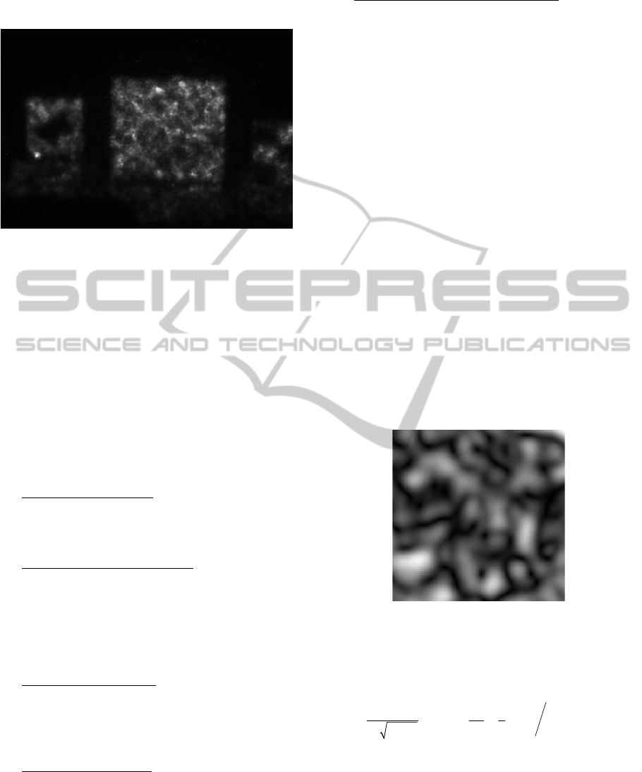
from the receiver close to the laser (two-way propa-
gation).
Figure 7: Two-way turbulence scintillations example at
SWIR wavelength, with C
n
2
=1.15⋅10
-14
. The image was
acquired at 1km range with a FOI developed Burst Illumi-
nation Ladar system.
A very accurate way to simulate this behavior of
the propagating beam is to use phase screens (An-
drews, 1998; Andrews, 2001). However, simulations
using phase screens are computationally very heavy.
We have near real-time demands on our simulations
and therefore we have chosen to use an approxima-
tion. In our simulation, the atmospheric effects are
divided into the following approximately indepen-
dent parts, where the theories are adapted from An-
drews (Andrews, 1998; Andrews, 2001).
A. The beam Broadening
, depends on turbulence
strength (
C
n
2
) and the wavelength. It affects the
spreading of the laser energy distribution that il-
luminates the scene.
B. The Turbulence Scintillations
. The engineering
approach used in the model is described in Sec-
tion 3.4.1. The scintillation pattern is primarily
based on a probability density function and a
cell size equation, which describes the spatial
pattern scale. The scintillations are multiplied to
the laser energy as can be seen in Figure 4.
C. The Aerial Attenuation
, which makes the pulse
energy decrease as the range increases. This is
due to smoke, fog, rain, and other particles in
the air, and is a factor in the laser radar equation
(3-1).
D. The Beam Wandering
. The laser beam optical
axis is randomly deflected by the turbulence in
the air as it propagates through the atmosphere.
This effect introduces a displacement of the
energy returning from the scene.
E. The Distortion and Blurring effect
, which can
be seen in the images in Figure 7. A simplified
way of modeling this is by using MTF (modula-
tion transfer function) to blur the image. This
corresponds to the MTF used in passive im-
agery, since it can be regarded as a one-way ef-
fect for the atmospheric propagation from the
target into the receiver optics. The MTF is ap-
plied by convolution.
The turbulence strength (
C
n
2
) varies slowly over
the day and reaches maximum at about noon, while
the lowest values occur close to sunset and sunrise.
This derives from the temperature gradient and wind
velocity, which usually are lower at night, especially
close to the shift between day and night. Close to the
ground the turbulence is stronger than high up in the
atmosphere.
3.4.1 Turbulence Scintillations
Statistically a distribution of intensities given as a
pdf (probability density function) can be determined
mathematically, according to equation (3-5). Even a
turbulence cell size can be determined. Using these
data a randomized turbulence scintillation pattern
can be determined, as the example in Figure 8.
Figure 8: Simulated turbulence scintillation example ac-
cording to equation (3-5).
The turbulence scintillation pdf during weak tur-
bulence conditions is described (Andrews, 2001) by
2
22
ln ln
2
ln
1
1
exp ln( ) 2
2
2
turb I I
av
I
S
P
S
S
σσ
πσ
⎛⎞
⎛⎞
⎜⎟
=−+
⎜⎟
⎜⎟
⋅
⎝⎠
⎝⎠
(3-5)
The pdf is based on the log-intensity variance,
σ
lnI
2
, which depends on the target resolution as seen
from the receiver, on the turbulence strength, and on
the light wavelength.
The turbulence cell radius,
ρ
l
, is determined in
relation to the spatial coherence radius of the current
turbulence condition (Andrews, 2001) as in equation
GRAPP 2011 - International Conference on Computer Graphics Theory and Applications
44
(3-6), where R is the range, k is the wave number
and
ρ
0
is the spatial coherence radius. This turbu-
lence cell radius is then used to spatially scale the
simulated turbulence scintillation.
()
2
0
1
l
Rk
Rk
ρ
ρ
=
+
(3-6)
To generate the spatial intensity distribution, as
the example in Figure 8, theory from Harris (Harris,
1995) is used as proposed by Letalick (Letalick,
2001). A randomized phase grid is generated, with
rectangular distribution (which is used by Goodman
(Goodman, 1984) in difference to Harris who uses
Gaussian distribution). This random field is multip-
lied by a Gaussian function corresponding to a field
distribution for the laser beam (TEM
00
). The Fourier
transform of the resulting matrix, the aperture func-
tion, gives the speckle field in the far field. By ad-
justing the spatial scale of the random noise and the
diameter of the Gaussian field distribution, different
scales and amplitudes for the speckle distribution
can be achieved. In this way the speckle field can be
matched to the probability density function in equa-
tion (3-5) and the turbulence cell size in (3-6).
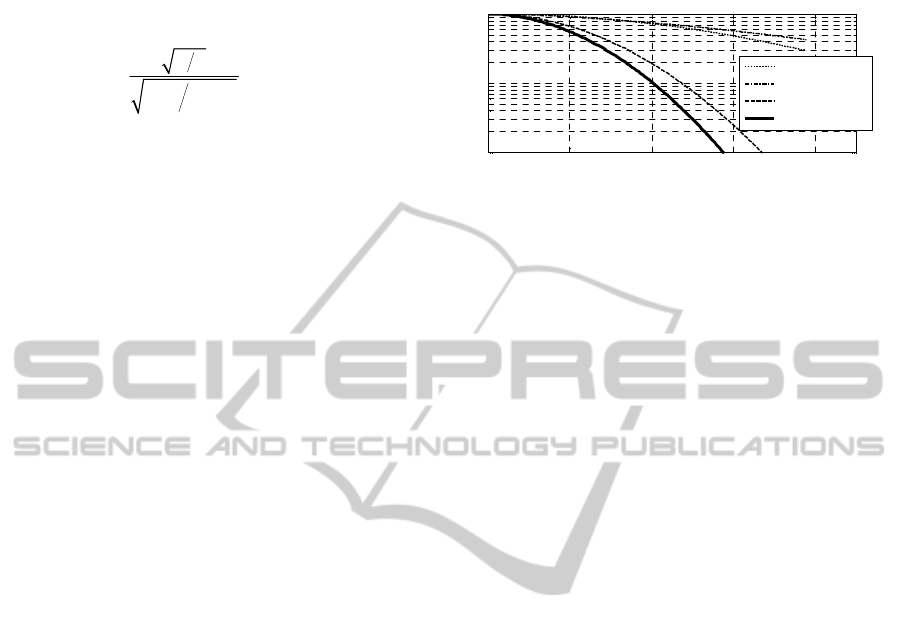
3.5 Sensor Data Degradation
Several parts of the model cover sensor data degra-
dation. The problem is not to simulate perfect undis-
turbed data, but to catch the most important degrad-
ing effects of the atmosphere, the scene and the sen-
sor.
There already exist well described theories for
sensor degradation of passive imaging, using MTF
(modulation transfer function). This MTF is applied
to passive imagery to decrease the effective resolu-
tion in a system, and can be separated into several
parts, where the total system MTF is a multiplication
of all separate MTFs;
MTF
speckle
for the speckle lim-
ited resolution,
MTF
opt
for the diffraction limited
(optical) resolution and
MTF
turb
for the turbulence
limited resolution. The MTF are applied on the sen-
sor data by convolution. As can be seen in Figure 9
the limiting MTF can be determined. The figure
shows one-dimensional MTFs, even though the
simulations are calculated in two dimensions, with
radial symmetry.
The receiver unit contains the conversion from
photons to a digital signal. This process introduces
noise in many ways, for instance by the A/D-
conversion quantization, the dark current back-
ground noise, and the read-out noise in the sensor
elements. This is modelled according to the model
structure in Figure 4.
0 20 40 60 80
10
-2
10
-1
10
0
spatial frequency [cyc/mrad]
Target speckle
Turbulence
Optics
Total
Figure 9: One system MTF example, where the optics is
the limiting MTF and affects the total MTF the most.
4 SPATIAL DISTRIBUTION
VALIDATION
This section describes the validation procedures and
results for the spatial energy distribution. The model
of the spatial energy distribution as a function of
different turbulence levels is compared to outdoor
measurements. First we validate the pdf of the en-
ergy distribution along with its cell size. Then we
estimate the accuracy in the total system noise.
The first part is done using measurements at 1km
range at weak and medium turbulence. The system
(used for both measurements and simulations) is a
burst illumination system at 532 nm. As can be seen
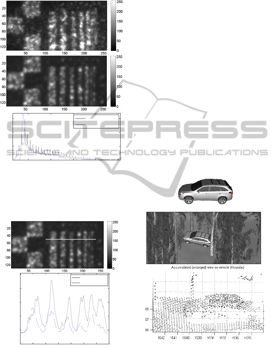
in Figure 10, the visual resemblance is quite good
between the measured (top row) and the simulated
(bottom row) images. The correspondence between
the energy distributions (histograms using all data in
the images) is shown in the bottom row of the figure,
where the solid line is the measured data, and the
dashed blue line is the simulated data. The cell size
is hard to measure exactly, but for this example the
simulated cell size was about 16 pixels and the
measured cell size was about 14 pixels, which we
consider to be within reasonable interval.
The same data collection was used for the second
part of the validation. Figure 11 show the chosen
profile that was compared for a set of data and cor-
responding simulations. The white line in the top
figure is chosen as the validation profile and it was
compared between the measured and the simulated
data as can be seen in the lower figure. The bias and
the gain was compared in the complete data set and
showed to fit quite well.
A RAY TRACING BASED MODEL FOR 3D LADAR SYSTEMS
45
50 100 150 200 250
0
500
1000
1500
Real data
Simulated data
Figure 10: Validation of spatial energy distribution, where
the top row is measured data on a reference board and the
middle row is the simulated corresponding data. The bot-
tom row shows a comparison between the energy distribu-
tions (histograms of all image data in the top images),
where the measured data is shown with solid black line
and simulated with dashed blue line.
0 20 40 60 80 100 120 140
0
50
100
150
200
250
Real data
Simulated data
Figure 11: One validation example, where the profile
marked with the white line in the top simulated image is
shown in the bottom. The true measured profile is shown
as the dashed line.
5 EXAMPLES
The flexible capabilities of the model are shown
with some examples; B
urst Illumination Ladar, 3D
Flash Ladar,
and Range Profiling Ladar.
5.1 Burst Illumination Ladar
Parameters for a Burst Illumination Ladar were set
up to validate the spatially high resolved turbulence
effects. The example in Figure 10 shows measured
data as well as simulated data from a Burst Illumina-
tion Ladar system with the target being a reference
resolution board at 1 km range.
5.2 3D Flash Ladar
The currently most advanced 3D imaging sensor
system, the 3D Flash Ladar, was modelled including
the range detection in each pixel, which resulted in a
set of points (128
×128) from each frame. The simu-
lations included a sensor movement during data cap-
ture, and the registered data can be seen in Figure
12.
Figure 12: Simulated 3D Flash Ladar example. The target
vehicle on top row is measured from a number of angles,
in the environment seen in the middle row, and the data is
globally registered in a common coordinate system, as
shown on bottom row.
GRAPP 2011 - International Conference on Computer Graphics Theory and Applications
46
The top row shows the target vehicle which was
placed on ground in a forested scene as seen on the
middle row. The bottom row shows the globally
registered points from five frames, collected from
separate viewing directions.
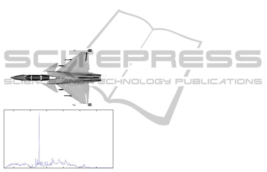
5.3 Range Profiling Ladar
The capability to simulate waveforms is illustrated
by this one dimensional simulation, where an air-
craft, JAS 39 Gripen, is flood illuminated with a
single laser beam, and all returning energy is col-
lected into one single waveform. The top row in
Figure 13 shows the target air craft that is illumi-
nated from the left and the bottom row shows the
returning echo.
150 200 250 300 350 400 45
0
Figure 13: Range profiling simulation of the JAS 39 Gri-
pen. The top row shows the target that is flood illuminated
with a laser from the left, and the returning echo wave-
form is shown below. Note the peak which corresponds to
the engine covers that were present at the aircraft model.
6 CONCLUSIONS
We have developed a model to simulate complex 3D
ladar systems. It is a model that combines imaging
of advanced scenario setups with atmospheric turbu-
lence modeling as well as allowing degrading sensor
effects to affect the resulting data. The simulation
framework is divided into four fundamental parts;
the scene, the laser source, the atmosphere and the
receiver.
Earlier models developed for ladar simulations
mostly lack the capability to simulate the atmos-
phere, or is not flexible enough to simulate several
types of systems. A key contribution with this paper
is therefore the atmospheric turbulence modeling
that fits a fairly simple scintillation pattern to the
advanced theory for laser beam propagation. We
have also presented that this turbulence modeling
can be applied to a complete system model that is
flexible and capable of modeling a number of sensor
system types. Finally, we have shown that the use of
advanced material reflections (BRDF) can be ap-
plied upon the commonly used ray tracing methods.
We have successfully validated some parts of the
model but also identified difficulties to validate the
atmospheric simulations due to some stochastically
varying entities. One important issue causing this
problem is the lack of measurement data, since some
atmospheric parameters uncontrollably varies during
acquisition. Another important issue is that the
knowledge about the parameters inside many of the
sensor systems are proprietary information and
therefore confidential.
REFERENCES
Andersson, P., 2006. Long range 3D imaging using range
gated laser radar images. Optical Engineering, 45.
Andrews, L. C. & Phillips, R. L., 1998. Laser Beam
Propagation through Random Media, Bellingham,
Washington, USA, SPIE Press.
Andrews, L. C., Phillips, R. L. & Hopen, C. Y., 2001.
Laser Beam Scinitillation with Applications, Belling-
ham, Washinton, USA, SPIE Press.
Budge, S., Leishman, B. & Pack, R., 2006. Simulation and
modeling of return waveforms from a ladar beam
footprint in USU LadarSIM. SPIE Defence & Security,
Laser Radar Technology and Applications XI, Or-
lando, FL, USA, 62140N.
Espinola, R. L., Teaney, B., Nguyen, Q., Jacobs, E. L.,
Halford, C. E. & Tofsted, D. H., 2007. Active imaging
system performance model for target acquisition. SPIE
Defense & Security Symposium, Infrared Imaging Sys-
tems: Design, Analysis, Modeling, and Testing XVIII,
Orlando, FL, USA, 65430T.
Goodman, J. W., 1984. Statistical Properties of Laser
Speckle Patterns. IN DAINTY, J. C. (Ed.) Topics in
Applied Physics: Laser Speckle and Related Phenom-
ena. 2nd ed., Springer-Verlag.
Grasso, R. J., Dippel, G. F. & Russo, L. E., 2006. A model
and simulation to predict 3D imaging LADAR sensor
systems performance in real-world type environments.
SPIE Atmospheric Optical Modeling, Measurement,
and Simulation II,, 63030H.
Grönwall, C., Steinvall, O., Gustafsson, F. & Chevalier,
T., 2007. Influence of laser radar sensor parameters on
range-measurement and shape-fitting uncertainties.
Optical Engineering, 46, 106201.
A RAY TRACING BASED MODEL FOR 3D LADAR SYSTEMS
47

Harris, M., 1995. Light-field fluctuations in space and
time Contemporary Physics, 36, 215-233.
Harvey, C., Wood, J., Randall, P., Watson, G. & Smith,
G., 2008. Simulation of a new 3D imaging sensor for
identifying difficult military targets. SPIE Defense &
Security Symposium, Laser Radar Technology and
Applications XIII, Orlando, FL, USA, 69500I.
He, X. E., Torrance, K. E., Sillion, F. X. & Greenberg, D.
P., 1991. A Comprehensive Physical Model for Light
Reflection. 18th annual conference on Computer
graphics and interactive techniques, 175-186.
Jelalian, A. V., 1992. Laser Radar System, Norwood, MA,
Artech House.
Letalick, D., Carlsson (later Grönwall), C. & Karlsson, C.,
2001. A speckle model for laser vibrometry. 11th Co-
herent laser radar conference, Great Malvern, UK,
44-47.
Moorhead, I. R., Gilmore, M. A., Houlbrook, A. W., Ox-
ford, D. E., Filbee, D. R., Stroud, C. A., Hutchings, G.
& Kirk, A., 2001. CAMEO-SIM: a physics-based
broadband scene simulation tool for assessment of
camouflage, concealment, and deception methodolo-
gies. Optical Engineering 40, 1896-1905.
Oren, M. & Nayar, S. K., 1995. Generalization of the
Lambertian model and implications for machine vi-
sion. International Journal of Computer Vision 14,
227-251.
Ortiz, S., Diaz-Caro, J. & Pareja, R., 2005. Radiometric
Modeling of a 3D Imaging Laser Scanner. SPIE Elec-
tro-Optical and Infrared Systems: Technology and
Applications II, 598709.
Phong, B. T., 1975. Illumination for Computer generated
pictures. Communications of the ACM, 18, 311-317.
Powell, G., Martin, R., Marshall, D. & Markham, K.,
2000. Simulation of FLIR and LADAR data using
graphics animation software. The Eighth Pacific Con-
ference on Computer Graphics and Applications,
Hong Kong, 126-134.
Savage, J., Coker, C., Edwards, D., Thai, B., Aboutalib,
O., Chow, A., Yamaoka, N. & Kim, C., 2006. Irma 5.1
multi-sensor signature prediction model. SPIE Defense
& Security Symposium, Targets & Backgrounds XII:
Characterization and Representation, Orlando, FL,
USA, 6239OC.
Savage, J., Coker, C., Thai, B., Aboutalib, O., Chow, A.,
Yamaoka, N. & Kim, C., 2007. Irma 5.2 multi-sensor
signature prediction model SPIE Defense & Security
Symposium, Modeling and Simulation for Military
Operations II, Orlando, FL, USA, 656403.
Savage, J., Coker, C., Thai, B., Aboutalib, O. & Pau, J.,
2008. Irma 5.2 multi-sensor signature prediction
model SPIE Defense & Security Symposium, Model-
ing and Simulation for Military Operations III, Or-
lando, FL, USA, 69650A.
Skolnik, M. I., 2008. Radar Handbook, New York, USA,
McGraw-Hill.
Steinvall, O., 1997. Theory for laser systems performance
modelling. Linköping, FOA. FOA-R--97-00599-612--
SE.
Steinvall, O., Olsson, H., Bolander, G., Carlsson (later
Grönwall), C. & Letalick, D., 1999. Gated Viewing
for target detection and target recognition. SPIE Laser
Radar Technology and Applications IV, Orlando, FL,
USA, 432-448.
Steinvall, O., 2000. Effects of target shape and reflection
on laser radar cross sections. Applied Optics, 39, 4381-
4391.
Torrance, K. E. & Sparrow, E. M., 1967. Theory for off-
specular reflection from roughened surfaces. Journal
of the Optical Society of America, 57, 1105-1114.
GRAPP 2011 - International Conference on Computer Graphics Theory and Applications
48
