
ELASTIC REGISTRATION OF EDGE SETS BY MEANS
OF
DIFFUSE SURFACES
With an Application to Embedding Purkinje Fiber Networks
Stefan F¨urtinger, Stephen Keeling
Institute for Mathematics and Scientific Computing, Karl–Franzens University, Graz, Austria
Gernot Plank, Anton J. Prassl
Institute for Biophysics, Medical University Graz, Graz, Austria
Keywords:
Elastic image registration, Edge sets, Diffuse surfaces, Purkinje Fibers, Endocardium.
Abstract:
In this work, edge sets are mapped one to the other by representing these zero area sets as diffuse images
which have positive measure supports that can be registered elastically. The driving application for this work
is to map a Purkinje fiber network in the epicardium of one heart to the epicardium of another heart. The
approach is to register sufficiently accurate diffuse surface representations of two epicardia and then to apply
the resulting transformation to the points of the Purkinje fiber network. To create a diffuse image from a given
edge set, a region growing method is used to approximate diffusion of brightness from an edge set to a given
point. To be minimized is the sum of squared differences of the registered diffuse images along with a linear
elastic penalty for the registration. A Newton iteration is employed to solve the optimality system, and the
degree of diffusion is larger in initial iterations while smaller in later iterations so that a desired local minimum
is selected by means of vanishing diffusion. Favorable results are shown for registering highly detailed rabbit
heart models.
1 INTRODUCTION
The heart is an electrically controlled mechanical
pump. It’s main function is to drive blood through
the circulatory system, thus providing oxygen and
metabolites to the organs. A well coordinated elec-
trical activation sequence is of vital importance for
allowing an energy-efficient mechanical contraction.
In the ventricles, the main pumping chambers of the
heart, the electrical impulse is conducted first via
the specialized conduction system, referred to as the
Purkinje system (PS).
The PS is a highly ramified network of thin cable-
like 1D structures which synchronizes ventricular ac-
tivation by quickly distributing the electrical impulse
to the endocardium, i.e. the surfaces of the ventric-
ular cavities. The PS is electrically isolated from
the ventricles except at discrete endpoints (Purkinje-
myocardial junctions) (Tranum-Jensen et al., 1991).
Transmission of the electrical signals at these discrete
junctional sites, referred to as Purkinje ventricular
junctions (PVJ) is essential to excite the ventricular
mass (Huelsing et al., 1998). A loss of electrical syn-
chronicity entails an impairment of the heart’s ability
to pump blood, which, ultimately, may even lead to
sudden cardiac death.
Despite recent advances, PS activity at the or-
gan level cannot be observed directly with currently
available experimental modalities. Computer models
quite naturally suggest themselves as a surrogate tech-
nique to bridge the gap between experimental obser-
vations, typically recorded at the epicardial surface of
the heart, and electrical events occurring within the
PS, at the ventricular epicardium or within the depth
of ventricular walls. Despite major recent advance-
ments in modeling technology (Prassl et al., 2009;
Plank et al., 2009), integrating topologically realistic
models of the PS with anatomically and functionally
realistic models of the ventricles remains to be chal-
lenging. Owing to the physiological importance of
the PS it is highly desirable to include the PS in com-
putational models.
The purpose of the present work was to develop
a mathematical framework which enables the map-
ping of the endocardial PS between different ven-
tricular surface geometries. In the absence of ex-
12
Fürtinger S., Keeling S., Plank G. and J. Prassl A..
ELASTIC REGISTRATION OF EDGE SETS BY MEANS OF DIFFUSE SURFACES - With an Application to Embedding Purkinje Fiber Networks.
DOI: 10.5220/0003322200120021
In Proceedings of the International Conference on Computer Vision Theory and Applications (VISAPP-2011), pages 12-21
ISBN: 978-989-8425-47-8
Copyright
c
2011 SCITEPRESS (Science and Technology Publications, Lda.)

perimental data, a literature-based PS (Vigmond and
Clements, 2007), constructed for the San Diego rabbit
heart model (Vetter and McCulloch, 1998), served as
reference topology. A recent anatomically highly re-
alistic model of rabbit ventricles (Bishop et al., 2010)
served as a target for developing and testing the map-
ping technique. Both models are shown in Figure 4.1.
We first seek a geometric transformation to match
the template heart model to a given reference model.
In the context of mathematical image processing this
can be seen as 3D registration problem. Once the
transformation is found it can be applied to map struc-
tures (like the PS) within the template model onto the
reference model. This approach guarantees that not
only topological features of the PS but also its relative
position to the ventricle are preserved and projected
onto the reference heart.
Given the sheer size of the models considered
here it would require a massive computational ef-
fort to calculate only simple transformations. Hence
we developed a method that is capable of comput-
ing even highly non-linear transformations in a rea-
sonable time while requiring only moderate compu-
tational resources. We performed a dimensional re-
duction of the problem by treating the 3D models as
sequence of 2D edges. This strategy reduces mem-
ory consumption considerably while simultaneously
allowing us to use very efficient techniques to solve
the occurring 2D registration problems.
2 EDGES AS BINARY IMAGES
We consider slices arising from cuts through (a) a re-
alistic model of rabbit ventricles (Bishop et al., 2010)
and (b) the San Diego rabbit heart (Vetter and McCul-
loch, 1998). Thus we have two-dimensional edge-sets
Γ
0
and Γ
1
and we assume that both edge-sets have
finite Hausdorff-measure H
1
(Γ
i
) < ∞ for i = 0,1.
Let Ω := [1,N]
2
⊂ R
2
with N ∈ N and let I
0
and I
1
be the characteristic functions of Γ
0
and Γ
1
respec-
tively. Then I
0
and I
1
can be interpreted as binary
images on Ω. The goal now is to find a displacement
w : R
2
→ R
2
such that I
0
(x + w(x)) ≈ I
1
(x) for all
x ∈ Ω. For the sake of brevity the argument of w is
omitted in the following.
One approach to the computation of the desired
displacement is to treat points on Γ
0
as if connected
to one another by elastic springs which are perturbed
minimally to meet the target set Γ
1
. However, be-
cause of the potentially very high computational com-
plexity of such a formulation, the approach used here
to match the edge sets is to embed them into images
which are then registered elastically. Elastic poten-
tial energy has been used by many authors to reg-
ularize image registration; see, e.g., (Peckar et al.,
1999), (Keeling and Ring, 2005) and particularly the
review in (Modersitzki, 2004). Such regularization
is particularly natural when used to register images
of tissues having undergone relatively small displace-
ments. However, in the present context, the required
displacement field is highly nonlinear, owing partly
to the complex geometry of the heart and partly to the
great difference in regularity of the two given edge
sets. Nevertheless elastic registration is employed
here, but with considerable precautions.
In addition to regularization, a notion of image
similarity must be selected for the image registration
problem at hand. Assuming that {I
i
}
i=0,1
⊂ L
2
(Ω)
one of the simplest distance measures (see for in-
stance (Fitzpatrick et al., 2000)) is the sum of squared
intensity differences (SSID) which in this case is
given by
1
2
Z
Ω
|I
0
(x+w) − I
1
(x)|
2
dx. (2.1)
However, in this form the approach is not feasible
for the problem: both Γ
0
and Γ
1
are null sets but
supp(I
i
) = Γ
i
for i = 0,1. Hence the trivial defor-
mation w ≡ 0 minimizes (2.1). Another in the con-
text of edges perhaps more natural approach to mea-
sure difference is employing the Hausdorff-distance
which is a popular tool in computer graphics and im-
age processing and mainly used for shape recognition
problems: In (Knauer et al., 2009) a method for mini-
mizing the Hausdorff-distance under translations and
rigid motions is developed. Though the proposed al-
gorithm is efficient it is limited to rigid transforma-
tions. In (Fuchs et al., 2009) an elastic deformation
distance in a shape space is introduced. However, cal-
culating the shortest path between shapes proved to
be computationally expensive. Another work (Droske
and Ring, 2006) developed a regularized shape gra-
dient descent algorithm within a level-set framework
for simultaneous registration and segmentation. How-
ever, the present problem still lacks sufficient struc-
ture to be treated directly by such approaches.
We present here a technique that combines the
simplicity of the SSID-measure (2.1) with the accu-
racy of the Hausdorff-distance. Instead of looking at
I
0
and I
1
directly we consider approximationsof edge-
sets by diffuse regions in images (a similar approach
is presented in (Yang et al., 2008)). Note that this
strategy is also employed by Ambrosio and Tortorelli
(Ambrosio and Tortorelli, 1990) in their approxima-
tion of the Mumford-Shah functional (Mumford and
Shah, 1989). Here, for ε > 0 define I
ε
i
for i = 0,1 by
ELASTIC REGISTRATION OF EDGE SETS BY MEANS OF DIFFUSE SURFACES - With an Application to
Embedding Purkinje Fiber Networks
13

I
ε
i
(x) :=
(
1− d
Γ
i
(x)/ε, if d
Γ
i
(x) ≤ ε,
0, otherwise.
(2.2)
The nonzero regions of I
ε
i
are diffuse extensions of
the edges Γ
i
. Since the distance function d
Γ
i
(x) can
be expensive to compute, I
ε
i
is calculated in practice
by a marching procedure in which the distance d
Γ
i
(x)
is approximated in terms of the number of march-
ing steps from the edge set Γ
i
to x. The extent of
this ”region-growing” depends on the magnitude of
ε: the effect looks like a silk painting of Γ
i
where ε
affects the duration of the brush touching the fabric.
From an image processing point of view this tech-
nique can be seen as distance transform. The use of
distance transforms in image registration is not new:
for instance in (Hill and Baldock, 2006) the authors
used constrained distances in the context of interac-
tive non-rigid registration. A variational approach to
match distance functions was presented in (Paragios
and Ramesh, 2002). Now we may use (2.1) on the
region-grown versions I
ε
i
of I
i
to obtain an adapted
distance measure
S
ε
(w) :=
1
2
Z
Ω
|I
ε
0
(x+ w) − I
ε
1
(x)|
2
dx. (2.3)
As indicated above, we assume that w is an elastic de-
formation; thus we define the following linear elastic
potential (see for instance (Modersitzki, 2004))
E(w) :=
λ
2
R
Ω
(∇· w)
2
dx+
µ
4
R
Ω
∇w
⊤
+ ∇w
2
F
dx,
(2.4)
where |·|
F
denotes the Frobenius-norm and µ and λ
are positive constants describing the elastic proper-
ties of the body, the so-called Navier–Lam´e constants.
Additively extending S
ε
by the linear elastic potential
E, ensures that among all solutions elastic deforma-
tions are favored. Hence we end up with the following
cost functional
J(w) := S
ε
(w) + E(w) (2.5)
for a fixed ε > 0. Assuming that w ∈ H
1
(Ω) the cost
J is well defined. Summarized we compute a registra-
tion by solving the following minimization problem
min
w∈H
1
(Ω)
J(w). (2.6)
Note that the images I
ε
i
vary with the value of ε.
We have proved the existence of a global minimizer
for (2.6) for each fixed ε as well as convergence of
these minimizers as ε → 0; however, these proofs are
not given here. Furthermore, we note that a global
minimizer for ε sufficiently small is essentially w= 0,
since (2.1) becomes negligible; thus, we are more
interested in the local minimizers introduced by our
novel vanishing diffusion strategy (see Algorithm 1
below) which starts with ε large enough that the de-
sired local minimum is dominant.
2.1 Optimality Conditions
We solve problem (2.6) by (formally) deducing the
corresponding Euler–Lagrange equations which we
linearize using Newton’s method (based on the work
in (Keeling, 2007)). To obtain the necessary optimal-
ity conditions for the optimization problem (2.6) we
compute the variational derivative of J in an arbitrary
direction v ∈ C
∞
(
¯
Ω)
δJ
δw
(w;v) :=
d
ds
J(w+ sv)
s=0
. (2.7)
To keep things clear we employ the linearity of the
Gˆateaux derivative and split the computation into two
parts. Starting with S
ε
we get
δS
ε
δw
(w;v) =
R
Ω
(I
ε
0
(x+ w) − I
ε
1
(x))∇I
ε
0
(x+ w) · vdx,
(2.8)
For E(w) we obtain
δE
δw
(w;v) =
R
Ω
µ
∇w
⊤
+ ∇w
:
∇v
⊤
+ ∇v
dx
+
R
Ω
λ(∇· w) (∇· v) dx, (2.9)
where : denotes a component-wisematrix scalar prod-
uct. The weak necessary condition for the minimiza-
tion of J is
δJ
δw
(w;v) =
δS
ε
δw
(w;v) +
δE
δw
(w;v) = 0, ∀v ∈ C
∞
(
¯
Ω).
(2.10)
To obtain a strong optimality formulation, we assume
first that w is sufficiently regular. By using partial in-
tegration we shift the derivatives from v to w and ap-
ply the fundamental Lemma of calculus of variations
to obtain the Euler–Lagrange equations of (2.6)
E w− f(x,w;I
ε
0
,I
ε
1
) =0, in Ω,
λn
ℓ
∇· w+ µ(∇w
ℓ
+ ∂
x
ℓ
w) · n =0, on ∂Ω,
(2.11)
where E is the elasticity operator defined by
E w := µ∆w+ (µ+ λ)∇(∇· w), (2.12)
and
f(x,w;I
ε
0
,I
ε
1
) := (I
ε
0
(x+ w) − I
ε
1
(x))∇I
ε
0
(x+ w),
(2.13)
is the driving force of the registration. Note that f is
the Gˆateaux derivative of the employed distance mea-
sure. This gives rise to some important observations:
if the force field f is small a slight deformation w is
enough to satisfy (2.11). Thus the distance measure
has to be sensitive enough to ”capture” differences
in the pathway of the edges Γ
i
. Hence a naive ap-
plication of the SSID-measure on the original binary
images I
i
is indeed not feasible for our problem: the
driving force f(x,w;I
0
,I
1
) is too small to yield a suffi-
ciently large deformation w to change the shape of Γ
0
visibly.
VISAPP 2011 - International Conference on Computer Vision Theory and Applications
14

However, at the same time the applied distance
measure has to be robust enough to ”ignore” minor
differences in the details of the edges Γ
i
in the pres-
ence of noise. Though the Hausdorff–distance gen-
erates a sufficiently large driving force for an elastic
registration it is very sensitive to noise: only modifi-
cations of the Hausdorff–distance-measure are capa-
ble of matching noisy image data (see e.g. (Sim et al.,
1999) or (Zhao et al., 2005)).
The technique of ”region-growing” proposed here
is able to satisfy both requirements: depending on the
choice of ε > 0 the broadening of the blurred edges
˜
Γ
ε
i
:= supp(I
ε
i
) for i = 0, 1 can be arbitrarily extended
thus provoking a large driving force f(x,w;I
ε
0
,I
ε
1
) if
the original edges Γ
i
differ significantly. On the other
hand the blurring effect or our ”region-growing” ap-
proach automatically smooths noisy edges by simul-
taneously preserving characteristic features. How-
ever, an inadequate choice of ε can lead to either ex-
cessive blurring and hence loss of important features
or insufficient enhancement of the edges and thus a
too small driving force f. Though the value of ε is
therefore critical the process of finding a suitable ε
is usually not too difficult. Nevertheless, in the fol-
lowing we present a solution strategy which is robust
against the choice of ε.
2.2 Solution Strategy
Since the Euler–Lagrange equations (2.11) are a sys-
tem of nonlinear partial differential equations (PDEs)
in w we employ Newton’s method on the functional J
which takes the form
δ
2
J
δw
2
(w
k
;v,δw
k
) = −
δJ
δw
(w
k
;v), ∀v ∈ C
∞
(
¯
Ω),
w
k+1
=w
k
+ τδw
k
,
(2.14)
where τ > 0 denotes a given step-size and k = 1,2,...
is the iteration index. We introduce the symmetriza-
tion
ˆ
∇I
ε
0
(x) := ∇I
ε
0
(x)∇I
ε
0
(x)
⊤
, (2.15)
and by employing again the linearity of the of the
Gˆateaux derivative we compute
δ
2
S
ε
δw
2
(w
k
;v,δw
k
) =
R
Ω
v
ˆ
∇I
ε
0
(x+ w
k
)δw
k
dx. (2.16)
By using the first variational derivative (2.9) of the
linear elastic potential we obtain further
δ
2
E
δw
2
(w
k
;v,δw
k
) =
R
Ω
µ(∇v
⊤
+ ∇v) : (∇δw
⊤
k
+ ∇δw
k
)
+
R
Ω
λ(∇· v)(∇· δw
k
)dx, (2.17)
Using again partial integration and the fundamental
Lemma of calculus of variations we arrive (under
stronger assumptions on the regularity of w) at the
following strong formulation:
(−E +
ˆ
∇I
ε
0
(x+ w
k
))δw
k
= E w
k
− f(x,w
k
;I
ε
0
,I
ε
1
)),
(2.18)
in Ω with boundary conditions
λn
ℓ
∇· w+ µ(∇w
ℓ
+ ∂
x
ℓ
w) · n = 0, (2.19)
on ∂Ω. Expressions (2.18)-(2.19) form the wanted
linear PDE-system for the unknown function δw
k
. We
could prove that the weak form (2.14) of the Newton
step admits an unique solution for each k if the im-
age I
ε
0
(x+w
k
) manifests sufficiently few symmetries.
Convergence of Newton’s method (2.14) for a fixed
ε > 0 and a suitable initial guess can be shown using
the Newton–Kantorovich Theorem (see e.g. (Ortega,
1968)).
3 NUMERICAL
APPROXIMATION
We will first introduce a discretization scheme for
the strong formulation (2.18)-(2.19) of the Newton
step and then explain the discrete realization of New-
ton’s method (2.14). We start by rewriting the Euler-
Lagrange equations (2.11). Let from now on w(x) :=
(u(x),v(x))
⊤
, and x = (x, y) ∈ Ω. Then we may
rewrite the elasticity operator E
E w =µ
∂
2
w
∂x
2
+
∂
2
w
∂y
2
+ (µ + λ)∇
∂u
∂x
+
∂v
∂y
=
(λ+2µ)
∂
2
∂x
2
+µ
∂
2
∂y
2
(λ+µ)
∂
2
∂x∂y
(λ+µ)
∂
2
∂x∂y
µ
∂
2
∂x
2
+(λ+2µ)
∂
2
∂y
2
!
(
u
v
)
=:
E
11
E
12
E
21
E
22
(
u
v
). (3.1)
For the sake of simplicity we drop the iteration in-
dex k here. Since we are working with digital im-
ages we define a grid Ω
h
:= {1,. .. ,N}
2
, where N
denotes the resolution of the images. We use an
unit step size h := 1, i.e. the width of a cell is one,
and employ standard central finite differences to dis-
cretize the Newton step (2.18)-(2.19). In particular
let j := ( j
1
,. .., j
N
) ∈ R
N
be an integer component
multi index, 1 := (1,. .., 1)
⊤
∈ R
N
and the cell cen-
troids be given by x
j
:= j, 1 ≤ j ≤ N · 1. We de-
note the array arising from evaluating e.g. u at each
grid point by u(Ω
h
) ∈ R
N×N
. Hence U
j
≈ u(x
j
) and
~u∈ R
N
2
denotes the vector of values {U
j
} correspond-
ing to the lexicographic ordering in which j
1
incre-
ments first from 1 to N, then j
2
and so on. Further, let
D(~u) ∈ R
N
2
×N
2
be the diagonal matrix arising from
situating the values {U
j
} along the diagonal accord-
ing to lexicographic ordering.
ELASTIC REGISTRATION OF EDGE SETS BY MEANS OF DIFFUSE SURFACES - With an Application to
Embedding Purkinje Fiber Networks
15

We start by discretizing the elasticity operator E .
We show for instance the discretization of E
11
near
the lower left corner of Ω
h
.
.
.
.
.
.
0 0 −2µ
0 8µ+4λ −4µ−4λ
0 0 −2µ
−2µ 0 −2µ
−4µ−4λ 16µ+8λ −4µ−4λ
−2µ 0 −2µ
·· ·
0 0 −2µ
0 2λ+4µ −2µ−2λ
0 0 0
−2µ 0 −2µ
−2µ−2λ 8µ+4λ −2µ−2λ
0 0 0
·· ·
(3.2)
The upper right block represents the stencil weights
for neighbors of a field cell. Similarly the other blocks
show for boundary cells the stencil weights for their
neighbors. With the same format we represent the
stencils of E
12
:
.
.
.
.
.
.
0 µ−λ −µ−λ
0 0 0
0 −µ−λ µ+λ
µ+λ 0 −µ−λ
0 0 0
−µ−λ 0 µ+λ
·· ·
0 µ−λ −µ−λ
0 µ+λ −µ+λ
0 0 0
µ+λ 0 −µ−λ
µ−λ 0 −µ−λ
0 0 0
·· ·
(3.3)
The stencils for E
22
and E
21
are constructed by ade-
quate copying and mirroring of (3.2) and (3.3) respec-
tively. This gives rise to matrices E
k.ℓ
∈ R
N
2
×N
2
with
1 ≤ k,ℓ ≤ 2 which form the discrete version of the
operator E under lexicographic ordering, i.e.
E (u(Ω
h
),v(Ω
h
)) ≈
E
11
~u+ E
12
~v
E
21
~u+ E
22
~v
, (3.4)
so that we may write
E~w :=
E
11
E
12
E
21
E
22
~u
~v
. (3.5)
Now we develop the discretization of the images I
ε
i
.
The discrete version
˜
I
1
∈ R
N×N
of I
ε
1
is readily es-
tablished by setting
˜
I
1,j
:= I
ε
1
(x
j
). Analogously we
set
˜
I
0,j
≈ I
ε
0
(x
j
+ w
j
). Note that for non-integer val-
ues of w a (multi)linear interpolation scheme has to
be applied to compute I
ε
0
(x+w) and ∇I
ε
0
(x+w). We
use bilinear interpolation to compute
˜
I
0,j
and intro-
duce the matrix
˜
I
0
∈ R
N×N
of values
˜
I
0,j
(if x+ w
lies outside of Ω we assign the extrapolation value
zero). Finally we approximate the gradient ∇I
ε
0
. Let
δh denote a fraction of the cell width h, i.e. δh :=
h/2 = 1/2. Employing this we get the increment of
I
ε
0
(x
j
+ w
j
) in x-direction to compute the following
discrete derivative
∂
∂x
I
ε
0
(x
j
+ w
j
) ≈
1
2δh
I
ε
0
(x
j
+ e
1
δh+ w
j
) (3.6)
−I
ε
0
(x
j
− e
1
δh+ w
j
)
=: δ
x
˜
I
0,j
,
where e
1
is the first unit vector in R
2
. Note that we
use again bilinear interpolation if I
ε
0
is evaluated at
non-grid points. Analogously we compute δ
y
˜
I
0,j
and
are finally ready to set up the discrete Newton step.
With : denoting again a componentwise matrix scalar
product let
G(
˜
I
0
) :=
D
−−−−−−→
δ
x
˜
I
0
:δ
x
˜
I
0
D
−−−−−−→
δ
x
˜
I
0
:δ
y
˜
I
0
D
−−−−−−→
δ
x
˜
I
0
:δ
y
˜
I
0
D
−−−−−−→
δ
y
˜
I
0
:δ
y
˜
I
0
!
∈ R
2N
2
×2N
2
,
(3.7)
and define
~
f :=
−−−−−−−−−→
(
˜
I
0
−
˜
I
1
) : δ
x
˜
I
0
−−−−−−−−−→
(
˜
I
0
−
˜
I
1
) : δ
y
˜
I
0
!
∈ R
2N
2
. (3.8)
Then the Newton step (2.18)-(2.19) is discretized by
−E+ G(
˜
I
0
)
δ~w = −E~w−
~
f, (3.9)
which is a linear equation system in the unknown
δ~w ∈ R
2N
2
3.1 The Discrete Newton Iteration
Now we want to establish a discrete version of New-
ton’s method (2.14) for the functional J. We use
~w
1
:= 0 ∈ R
2N
2
as initial guess and employ the discrete
Newton step (3.9) to obtain the following iteration
(
−E+ G(
˜
I
0,k
)
δ~w
k
= − E~w
k
−
~
f
k
,
~w
k+1
=~w
k
+ τ
k
δ~w
k
,
k = 1, 2,...
(3.10)
Note that the discrete gradient G(
˜
I
0,k
) and the discrete
force
~
f
k
depend on the current value of ~w
k
hence they
have to be updated at each iteration.
We use a backtracking-like line search to deter-
mine the step size τ
k
. We establish a discrete approxi-
mation J
h
of the cost functional J and determine τ
k
as
follows:
τ
k
=min
τ∈T
J
h
(~w
k
+ τδ~w
k
),
T :=
τ =
2ℓ
L
|ℓ = 1, ... ,L
,
(3.11)
where ~w
k
denotes the current iterate and δ~w
k
the cur-
rently computed Newton direction. Note that this
line-search algorithm determines the optimal step-
size on the interval [2/L,2] hence in contrary to clas-
sic backtracking approaches (Dennis and Schnabel,
1983) step sizes larger than one can be chosen. This
method has proven to provide good performance and
less total computational cost than standard Armijo–
Goldstein or Wolfe–Powell techniques (Nocedal and
Wright, 2000). Since L > 0 is not chosen to be partic-
ularly large only few evaluations of J
h
are computed
to obtain τ
k
and the computation of J
h
does not in-
volve the expensive calculation of the discrete gradi-
ent G(
˜
I
0,k
).
VISAPP 2011 - International Conference on Computer Vision Theory and Applications
16

We use a relative stopping criterion in the New-
ton iteration (3.10). Note that the right hand side of
the Newton step (3.9) corresponds to the discretized
Euler–Lagrange equations (2.11) of the original min-
imization problem (2.6). Hence we want the residual
r
k
:= −E~w
k
−
~
f
k
to be ”small” and thus define the rel-
ative residual r
b
:= |r
k
|/|r
1
|. Additionally we com-
pute the relative change of the iterates r
e
:= |~w
k
−
~w
k−1
|/|~w
k
| (where r
e
:= 0 if |~w
k
| = 0) and combine
these two notions in a stopping criterion.
As mentioned above the choice of ε may have
negative effects on the outcome of the registration.
Whereas it is usually not too difficult to avoid too
small values of ε it is very hard to give an upper
bound for ε beforehand. However, a value of ε too
large leads to excessively blurred approximations I
ε
i
of I
i
and hence a loss of potentially important features
of the original edges Γ
i
. Hence we want the solu-
tion strategy of the registration problem (2.6) to be
robust against the choice of ε. To account for the in-
troduced approximation error we augment Newton’s
method (3.10) with an outer iteration in which we re-
duce blurring. We compute a rough solution ~w
⋆
of
(3.10) by using a low number of maximal iterations
k
max
. To reduce blurring in the images we compute
the element-wise-squared of
˜
I
ε
i
which accentuates the
original edge sets Γ
i
in contrast to their blurred sur-
roundings. Then we restart Newton’s method with the
images
˜
I
ε
i
(x
j
)
2
, ~w
1
= ~w
⋆
and increase k
max
. We repeat
this procedure K times such that the squared images
are sufficiently close approximations to the original
images, i.e
˜
I
ε
i
(x
j
)
2
K
≈ I
i
(x
j
). To fix ideas we sum-
marize this method in Algorithm 1.
Algorithm 1: Iterative method to solve the elastic registra-
tion problem (2.6).
Choose ε > 0, k
inc
∈ N : k
inc
≥ 2, tol > 0 and ~w ∈ R
2N
2
.
1. Given the edge-sets Γ
0
and Γ
1
embed them in the center
of images I
0
and I
1
.
2. Compute diffuse versions I
ε
i
o
f I
i
.
3.
for
κ = 1
to
K
(a) Set k
max
= k
inc
· κ
(b) Compute ~w
⋆
according to (3.10) using the line search
strategy (3.11) until either min(r
b
,r
e
) < tol or k >
k
max
.
(c) Set
˜
I
ε
i
(x
j
) :=
˜
I
ε
i
(x
j
)
2
and ~w
1
= ~w
⋆
.
4.
end
5. Set ~w = ~w
⋆
.
The centering of the edges as stated in Algo-
rithm 1 is an important pre-registration step: if the
edges are not centered within the images I
i
the diffuse
extensions of Γ
i
created by (2.2) may intersect image
boundaries. This would greatly impair the computa-
tion of the deformation ~w at the boundary since mass
having diffused over the boundary cannot be matched
with its natural counterpart in the other image. More-
over, if both edges Γ
0
and Γ
1
share roughly the same
area of the images I
0
and I
1
respectively the deforma-
tion field does not have to account for large transla-
tions within the image domain.
Altogether this approach has proven itself in prac-
tice: since the minimization problem (2.6) is only
approximately solved for blurred versions
˜
I
ε
i
of I
i
in
the beginning, a rough initial deformation field is ob-
tained that captures only global deformations in I
0
.
By successively deblurring the images
˜
I
ε
0
and
˜
I
ε
1
the
pathway of the original edge sets Γ
i
takes shape again,
and the deformation ~w is updated to capture local fea-
tures of the edges.
4 COMPUTATIONAL RESULTS
All computations were carried out in MATLAB
TM
2009b running on a Dell Optiplex 745 equipped with
8 GB of RAM. The used operating system was open-
SUSE 11.2 (64bit, kernel 2.6.31.12-0.2).
We want to apply the solution strategy developed
in the previous section to register the San Diego rab-
bit heart (Vetter and McCulloch, 1998) (referred to
as “TBunnyC” in the following) to an anatomically
highly realistic model (Bishop et al., 2010) (called
“Oxford-heart” from now on). Both models are
shown in Figure 4.1. The basic idea is to slice up the
3D models which gives rise to 2D edges. Then each
slice is registered consecutively by employing Algo-
rithm 1. The registered slices are assembled again to
obtain a 3D representation of the results. Finally the
deformation fields computed for each slice are used
to map a literature-based Purkinje fiber network (Vig-
mond and Clements, 2007) onto the endocardium of
the Oxford-heart.
The measuring unit of the models is µm; hence,
we rescaled the large values in the models to reduce
the size of the arising linear systems in the registra-
tion. Further, to obtain a maximal spatial ”overlap”
we translated the models. Then we ”cut” the 3D mod-
els to obtain 2D edges. To ensure a clear differen-
tiation between left and right cavity we separate the
3D heart models accordingly. We chose the z-axis as
cutting direction which seems to be a natural choice
once left and right cavities are considered separately.
Due to the fact that the grid points are not equally dis-
tributed on regular xy-planes in vertical direction we
have to divide the models into layers of finite thick-
ness, particularly with a thickness of 250µm. The
ELASTIC REGISTRATION OF EDGE SETS BY MEANS OF DIFFUSE SURFACES - With an Application to
Embedding Purkinje Fiber Networks
17

(a) (b)
Figure 4.1: The given 3D heart models: (a) The San Diego rabbit heart (Vetter and McCulloch, 1998) ”TBunnyC” (29 394
points) and (b) the anatomically highly realistic model (Bishop et al., 2010) ”Oxford Heart” (258 178 points).
(a)
(b) (c)
Figure 4.2: Illustration of the dissection of the 3D heart
models. Shown is the left cavity of the TBunnyC model.
First the model is cut in horizontal direction (a) to gener-
ate a 2D edge set (b). We center the image and apply our
region-growing algorithm (c).
wanted 2D edges arise from shrinking the thickness
until the slice becomes an xy-plane.
Having generated a series of slices we are ready
to apply Algorithm 1. Each slice is a sparse dou-
ble MATLAB matrix of size N × N. We apply two
preprocessing steps: for each slice we first center
the edges within the images and second we employ
our ”region-growing” algorithm to obtain blurred ap-
proximations I
ε
i
. We approximate the distance func-
tion d
Γ
i
used in the definition (2.2) of I
ε
i
by the fol-
lowing marching scheme: Each non-zero entry of I
i
is multiplied by N and added to its 3 × 3 neighbor-
hood. This procedure is repeated until either the edge
set ”outgrows” the image or a maximal number of
iterations has been exceeded. An exemplary result
of this region-growing is depicted in Figure 4.2(c).
This way we generated two image series: the blurred
slices of the 3D model TBunnyC
I
ε,m
0
M
m=1
which
serve as template image stack and the blurred cuts of
the Oxford-heart
I
ε,m
1
M
m=1
which form the reference
stack. Thus we want to find elastic deformations w
m
so that I
ε,m
0
(x+ w
m
) ≈ I
ε,m
1
(x) for m = 1,. .., M. This
is achieved by employing a MATLAB-implementation
of the augmented Newton method depicted in Algo-
rithm 1. A list of all used parameters and their values
is given in Table 4.1. The discrete Newton step (3.9) is
solved using the inbuilt MATLAB-function
mldivide
(”backslash”). To utilize memory efficiently the coef-
ficient matrices in each Newton step are sparse double
MATLAB matrices. Finally we apply the computed
deformations w
m
to the original images I
m
0
to register
the edges Γ
m
0
to Γ
m
1
. Figure 4.3 sketches the proce-
dure. Figure 4.4 shows the 3D reconstruction of the
registered TBunnyC slices in comparison to the 3D
reference, i.e. the Oxford heart, for both left and right
cavities.
Having registered each slice of the left and right
cavities we want to utilize the computed deformation
fields to map an artificial Purkinje fiber network given
for the TBunnyC model onto the Oxford heart. The
VISAPP 2011 - International Conference on Computer Vision Theory and Applications
18

(a)I
ε
0
(b)I
ε
0
(x+ w)
2
K
(c)I
0
(x+ w)
(d)I
ε
1
(e)I
ε
1
(x)
2
K
(f)I
1
(x) (g)w(x)
Figure 4.3: The different stages of Algorithm 1 for the template image I
0
(top row) and the reference image I
1
(bottom
row). Panels (a) and (d) show the centered and region grown versions of the images. Panel (b) presents the resulting image
I
ε
0
(x+ w)
2
K
after completion of Algorithm 1 versus the final reference I
ε2
K
1
(x) (e). Panel (c) depicts the original image I
0
after application of the computed transformation w versus the original target I
1
(f). Panel (g) shows the computed deformation
field w(x).
Table 4.1: The used parameters.
Parameter Value Meaning
λ 1e-2 see (2.4)
µ 1e-2 see (2.4)
L 10 see (3.11)
tol 1e-3 see Algorithm 1
K 4 see Algorithm 1
k
inc
5 see Algorithm 1
PS was given as list of Cartesian coordinates of 832
points (414 points for the left, 418 points for the right
cavity respectively) representing the spatial locations
of the nodes of a 3D graph. Figure 4.5 shows the
Purkinje fiber network in the TBunnyC model in com-
parison to the registered network in the Oxford heart.
5 DISCUSSION
AND CONCLUSIONS
The artificial PS considered here was modeled to be a
subset of the TBunnyC model. Hence we may safely
assume that the computed deformations constitute a
suitable mapping for projecting the network nodes
from the TBunnyC model onto the Oxford heart. The
application required the registered network to be a
subset of the Oxford heart. This requirement to-
gether with the sheer number of network nodes ren-
dered it impossible to construct an affine linear map-
ping to roughly project the nodes into a proximity of
the Oxford endocardium and successively correcting
the spatial position of each individual point. More-
over, the complexgeometry of the Oxford heart which
differs significantly from the topology of the TBun-
nyC model proved to be captured adequately only by
elastically deforming the TBunnyC endocardial walls.
Hence the computed elastic deformations guarantee
that despite even large differences in the endocardial
geometries of both models the artificial Purkinje fiber
network is mapped sufficiently close to the Oxford
endocardium. Post-processing can be used to project
nodes onto the nearest facet.
Though our results have been positively evalu-
ated by experts, the lack of experimental observations
makes a rigorous validation difficult. While our 2D
approach depends strongly upon the preregistrations
performed in 3D and in 2D, this dependence might
be relaxed by a full 3D registration at considerably
higher cost. Our simulations confirmed that separat-
ing the cavities of the heart models is crucial. This can
be seen rather easily by looking at Figure 4.1: we see
that cutting the hearts in vertical direction gives rise
to slices which contain edges from both the left and
right cavities. This fact seriously impairs the outcome
of the registration: depending on the choice of the
Navier–Lam´e constants and the proximity of the cavi-
ties the computed deformationfields ”pull” edges cor-
responding to the left cavity to an edge arising from
a cut through the right cavity and vice versa. Despite
numerous tests using different parameter values and
ELASTIC REGISTRATION OF EDGE SETS BY MEANS OF DIFFUSE SURFACES - With an Application to
Embedding Purkinje Fiber Networks
19
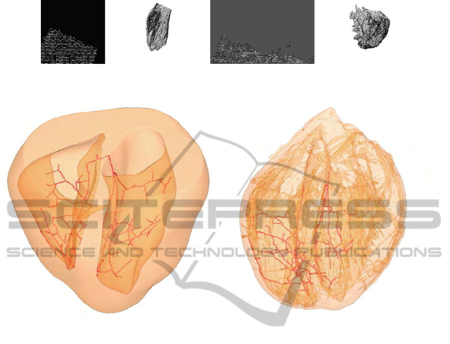
Figure 4.4: 3D Reconstruction of the registered TBunnyC slices for the left (a) and right (c) cavity vs the left (b) and right (d)
cavity of the reference Oxford heart.
(a) (b)
Figure 4.5: The artificial Purkinje fiber network in the TBunnyC model (a) and the registered network in the Oxford heart (b).
cutting directions this undesirable effect could not be
completely eradicated. Hence we separated the 3D
hearts into left and right cavities.
Despite the application presented here our method
proved to be a highly efficient and reliable technique
to register 2D edges. In contrast to previously devel-
oped techniques involving the Hausdorff-distance our
approach is computationally cheap and not limited to
rigid transformations. The approximation of edges
by diffuse surfaces allows us to use a standard SSID
distance-measure which is simple to compute and can
be easily extended by an elastic penalizer to account
for nonlinear deformations. Due to the plain structure
of the associated cost functional the derivation of nec-
essary optimality conditions by means of variational
calculus is straight forward. The use of variational
derivatives further enables us to employ fast and the-
oretically well-founded optimization routines such as
Newton’s method. Furthermore, the driving force of
the registration can be quickly evaluated and is easy
to interpret. In relation to other works employing
blurring strategies in registration problems we note
that our novel vanishing diffusion strategy described
in Algorithm 1 ensures robustness of the proposed
method.
ACKNOWLEDGEMENTS
All authors are supported by the Austrian Science
Fund Fond zur F
¨
orderung der Wissenschaftlichen
Forschung (FWF) under grant SFB F032 (“Mathe-
matical Optimization and Applications in Biomedical
Sciences” http://math.uni-graz.at/mobis).
REFERENCES
Ambrosio, L. and Tortorelli, V. (1990). Approximation of
functionals depending on jumps by elliptic function-
als via γ-convergence. Communications on Pure and
Applied Mathematics, 43:999–1036.
Bishop, M. J., Plank, G., Burton, R. A., Schneider, J. E.,
Gavaghan, D. J., Grau, V., and Kohl, P. (2010). De-
velopment of an anatomically detailed MRI-derived
rabbit ventricular model and assessment of its impact
VISAPP 2011 - International Conference on Computer Vision Theory and Applications
20

on simulations of electrophysiological function. Am J
Physiol Heart Circ Physiol, 298(2):H699–718.
Dennis, J. and Schnabel, R. (1983). Numerical Methods
for Unconstrained Optimization and Nonlinear Equa-
tions. Prentice–Hall, Englewood Cliffs, NJ,.
Droske, M. and Ring, W. (2006). A mumford-shah level-
set approach for geometric image registration. SIAM
Journal of Applied Mathematics, 66(6):2127–2148.
Fitzpatrick, J., Hill, D., and Maurer, C. (2000). Image Reg-
istration, Medical Image Processing, volume 2, chap-
ter 8 of the Handbook of Medical Imaging. SPIE
Press.
Fuchs, M., J¨uttler, B., Scherzer, O., and Yang, H. (2009).
Shape metrics based on elastic deformations. J. Math.
Imaging Vis., 35(1):86–102.
Hill, W. and Baldock, R. A. (2006). The constrained dis-
tance transform: Interactive atlas registration with
large deformations through constrained distances. In
DEFORM’06 - Workshop on Image Registration in
Deformable Environments.
Huelsing, D. J., Spitzer, K. W., Cordeiro, J. M., and Pol-
lard, A. E. (1998). Conduction between isolated rabbit
purkinje and ventricular myocytes coupled by a vari-
able resistance. Am J Physiol, 274(4 Pt 2):H1163–
H1173.
Keeling, S. and Ring, W. (2005.). Medical image regis-
tration and interpolation by optical flow with maximal
rigidity. Journal of Mathematical Imaging and Vision,
23(1):47–65.
Keeling, S. L. (2007). Generalized rigid and generalized
affine image registration and interpolation by geomet-
ric multigrid. Journal of Mathematical Imaging and
Vision, 29:163–183.
Knauer, C., Kriegel, K., and Stehn, F. (2009). Minimizing
the weighted directed hausdorff distance between col-
ored point sets under translations and rigid motions. In
FAW ’09: Proceedings of the 3d International Work-
shop on Frontiers in Algorithmics, pages 108–119,
Berlin, Heidelberg. Springer-Verlag.
Modersitzki, J. (2004). Numerical Methods for Image Reg-
istration. Oxford Science Publications.
Mumford, D. and Shah, J. (1989). Optimal approximations
by piecewise smooth functions and associated varia-
tional problems. Communications on Pure and Ap-
plied Mathematics, 42(5):577–685.
Nocedal, J. and Wright, S. (2000). Numerical Optimization.
Springer.
Ortega, J. M. (1968). The newton–kantorovich theorem.
The American Mathematical Monthly, 75(6):658–
660.
Paragios, N. and Ramesh, M. R. V. (2002). Matching dis-
tance functions: A shape-to-area variational approach
for global-to-local registration. In Proceedings of the
7th European Conference on Computer Vision-Part II.
Peckar, W., Schn¨orr, C., Rohr, K., and Stiehl, H. S. (1999).
Parameter-free elastic deformation approach for 2d
and 3d registration using prescribed displacements. J.
Math. Imaging Vis., 10(2):143–162.
Plank, G., Burton, R. A., Hales, P., Bishop, M., Mansoori,
T., Bernabeu, M. O., Garny, A., Prassl, A. J., Bol-
lensdorff, C., Mason, F., Mahmood, F., Rodriguez, B.,
Grau, V., Schneider, J. E., Gavaghan, D., and Kohl,
P. (2009). Generation of histo-anatomically repre-
sentative models of the individual heart: tools and
application. Philos Transact A Math Phys Eng Sci,
367(1896):2257–92.
Prassl, A. J., Kickinger, F., Ahammer, H., Grau, V., Schnei-
der, J. E., Hofer, E., Vigmond, E. J., Trayanova,
N. A., and Plank, G. (2009). Automatically gener-
ated, anatomically accurate meshes for cardiac elec-
trophysiology problems. IEEE Trans Biomed Eng,
56(5):1318–30.
Sim, D.-G., Kwon, O.-K., and Park, R.-H. (1999). Object
matching algorithms using robust hausdorff distance
measures. IEEE Transactions on Image Processing,
8(3):425–429.
Tranum-Jensen, J., Wilde, A. A., Vermeulen, J. T., and
Janse, M. J. (1991). Morphology of electrophysiolog-
ically identified junctions between purkinje fibers and
ventricular muscle in rabbit and pig hearts. Circ Res,
69(2):429–437.
Vetter, F. and McCulloch, A. (1998). Three-dimensional
analysis of regional cardiac function: a model of rab-
bit ventricular anatomy. Prog Biophys Mol Biol, 69(2-
3):157–83.
Vigmond, E. J. and Clements, C. (2007). Construction of a
computer model to investigate sawtooth effects in the
purkinje system. IEEE Trans Biomed Eng, 54(3):389–
399.
Yang, S., Kohler, D., Teller, K., Cremer, T., Le Baccon,
P., Heard, E., Eils, R., and Rohr, K. (2008). Nonrigid
registration of 3-d multichannel microscopy images of
cell nuclei. IEEE Transactions on Image Processing,
17:493–499.
Zhao, C., Shi, W., and Deng, Y. (2005). A new hausdorff
distance for image matching. Pattern Recognition Let-
ters, 26(5):581–586.
ELASTIC REGISTRATION OF EDGE SETS BY MEANS OF DIFFUSE SURFACES - With an Application to
Embedding Purkinje Fiber Networks
21
