PERSPECTIVE-THREE-POINT (P3P) BY DETERMINING

THE SUPPORT PLANE

Zhaozheng Hu

Graduate School of Informatics, Kyoto University, Kyoto 606-8501, Japan

College of Information Science and Technology, Dalian Maritime University, Dalian 116026, China

Takashi Matsuyama

Graduate School of Informatics, Kyoto University, Kyoto 606-8501, Japan

Keywords: Perspective-Three-Point (P3P), Support plane, Plane normal, Maximum likelihood.

Abstract: This paper presents a new approach to solve the classic perspective-three-point (P3P) problem. The basic

conception behind is to determine the support plane, which is defined by the three control points.

Computation of the plane normal is formulated as searching for the maximum likelihood on the Gaussian

hemisphere by exploiting the geometric constraints of three known angles and length ratios from the control

points. The distances of the control points are then computed from the normal and the calibration matrix by

homography decomposition. The proposed algorithm has been tested with real image data. The computation

errors for the plane normal and the distances are less than 0.35 degrees, and 0.8cm, respectively, within

1~2m camera-to-plane distances. The multiple solutions to P3P problem are also illustrated.

1 INTRODUCTION

Perspective-n-Point (PnP) is a classic problem in

computer vision field and has important applications

in vision based localization, object pose estimation,

and metrology, etc (Fischler et al., 1981, Gao et al.,

2003, Moreno-Noguer et al., 2007, Vigueras et al.,

2009, Wolfe et al., 1991, Wu et al., 2006, and

Zhang, et al., 2006). The task of PnP is to determine

the distances between camera and a number of

points (n control points), which are well known in an

object coordinate space, from the image, that is

taken by a calibrated camera. Existing PnP

researches mainly focused on n=3, 4, 5 cases, also

known as P3P, P4P, and P5P problems. Among

them, P3P (n=3) problem requires the least

geometric constraints and it is also the minimum

point subset that yield finite solutions. Existing P3P

researches can be classified into two categories.

Researches in the first category try to solve P3P

using different approaches, such as algebraic,

geometric approaches, etc (Fischler et al., 1981,

Moreno-Noguer et al., 2007, Vigueras et al., 2009,

and Wolfe et al., 1991). Researches in the second

one try to classify the solutions and study the

distribution of multiple solutions (Fischler et al.,

1981, Gao et al., 2003, Wolfe et al, 1991, Wu et al.,

2006, and Zhang, et al., 2006). The P3P problem

was first proposed in (Fischler et al., 1981), which

proves that P3P has at most four positive solutions.

Wolfe et al. gave geometric explanation of P3P

solution distribution and showed that most of the

time P3P problem gives two solutions (Wolfe et al,

1991). Gao et al. gave a complete solution set of the

P3P problem (Gao et al., 2003). More work on P3P

and on the general PnP problems can be found in the

literatures (Moreno-Noguer et al., 2007, Vigueras et

al., 2009, Wu et al., 2006, and Zhang, et al., 2006).

The work in the paper falls into the first

category, which tries to address P3P by determining

the support plane. We show that the key to P3P

problem is to compute the plane normal.

Computation of plane normal is formulated as a

maximum likelihood problem from the geometric

constraints of three control points so that the normal

is computed by searching for the maximum

likelihood on the Gaussian hemisphere. Once the

normal is calculated, we can determine the support

plane, compute the distances of the control points to

the camera, and solve the P3P problem.

119

Hu Z. and Matsuyama T..

PERSPECTIVE-THREE-POINT (P3P) BY DETERMINING THE SUPPORT PLANE.

DOI: 10.5220/0003320301190124

In Proceedings of the International Conference on Computer Vision Theory and Applications (VISAPP-2011), pages 119-124

ISBN: 978-989-8425-47-8

 2011 SCITEPRESS (Science and Technology Publications, Lda.)

2 PLANE RECTIFICATION

FROM HOMOGRAPHY

Under a pin-hole camera model, a 3D point with the

homogeneous coordinates

[]

ZYXM 1=

projected onto an image plane, with the image

[]

vum 1=

given by the following imaging

process (Hartley & Zisserman, 2000)

[][][ ]

ZYXtRKvu 11 ×≅

(1)

where

≅

means equal up to a scale,

is the

calibration matrix,

and

are the rotation matrix

and the translation vector, respectively.

Assume a reference plane coincides with the X-

O-Y plane (

0=Z ) of the world coordinate system.

We can derive the relationship between a 2D point

[]

YXM 1=

on the plane

and its image

from Eq. (1) as follows (Zhang, 2000)

[]

[

]

YXtrrKm 1

×≅



(2)

where

is the i

column of the rotation matrix.

Hence,

and

are related by a 3×3 matrix,

called homography. It is possible to compute the

homography from the vanishing line or plane

normal, and the camera calibration matrix, according

to the stratified reconstruction theory. The

computation details are referred to (Hartley &

Zisserman, 2000, Liebowitz & Zisserman, 1998).

Once the homography is determined, we can use

it to rectify the physical coordinates of points on the

reference plane from Eq. (2) as follows

mHM

1−

≅

(3)

Once the coordinates are rectified from Eq. (3),

more planar geometric attributes can computed, such

as distance, length ratio, angle, shape area,

curvature, etc. These computed geometric attributes

are defined as rectified geometric attributes.

3 THE PROPOSED ALGORITHM

3.1 P3P from Support Plane

The formulation of P3P problem is referred to

(Fischler et al., 1981, and Wolfe et al., 1991), which

states that “given the camera calibration matrix, the

relative positions of three points, also called control

points, and the images of the control points on the

imaging plane, compute the distance of each control

point to the camera center”.

The three control points define an unique support

plane. If the plane is well determined, e.g., the

normal and the distance, we can compute its

intersections with the re-projection rays, which can

be computed from the images of the control points

and calibration matrix. Hence, the 3D coordinates of

the intersections (also control points) are determined

readily, and the distances are thereafter computed.

According to stratified reconstruction theories, the

key to determine a plane is the normal (Hartley &

Zisserman, 2000, Liebowitz & Zisserman, 1998).

Once the plane normal is calculated, a metric

reconstruction of a plane is ready by using the

calibration matrix (Hartley & Zisserman, 2000, and

Liebowitz & Zisserman, 1998). An actual distance

e.g., distance between two arbitrary control points,

can upgrade a metric reconstruction to Euclidean

one. As a result, the distance of the plane is

computed readily. Therefore, the key to P3P is to

compute the normal of the support plane.

3.2 Plane Normal Computation

3.2.1 Basic Geometric Constraints from

Three Control Points

Let

321

,, PPP

be the three control points, from

which, we can compute three lengths in-between as

213

312

321

PPD

−=

(4)

where

•

is Euclidean distance operator. Hence,

three length ratios can be derived as

213

312

321

(5)

We can also compute three angles from the

triangle defined by the three points as

(

)

(

)

(

)

()

2/cos

DDDDD

××−+=

(6)

From Eq. (5) and Eq. (6), we can derive six

geometric constraints

(

)

6,2,1 "=iC

on the plane

normal from the three control points as follow

VISAPP 2011 - International Conference on Computer Vision Theory and Applications

120

(){}()

6,2,1| "=== iuNSCC

iii

(7)

where

is the geometric attribute of the i

constraint, e.g., the value of

, as specified

in Eq. (5) and Eq. (6), and

()

is the rectified

geometric attribute, which can be computed from

homography, given the plane normal.

3.2.2 Maximum Likelihood Model

We try to compute the plane normal from the six

geometric constraints, as specified in Eq. (7) above.

This can be formulated as to maximize the following

conditional probability (Hu & Matsuyama, 2010),

which is given as follows

()

621

,,|maxarg CCCNP

(8)

where

N is the plane normal to compute.

Therefore, Eq. (8) tries to compute the plane normal

with the highest probability, given the six geometric

constraints from the control points. Actually, it is

difficult to solve Eq. (8) directly. By using Bayes’

rule, we can re-arrange Eq. (8) as

()

()()

()

621

|,,

,,|

CCCP

NPNCCCP

CCCNP

(9)

where

()

NCCCP |,,

611

is known as the

likelihood,

()

and

()

621

,, CCCP "

are the prior

probabilities for the plane normal directions and

geometric constraints, respectively. Assume that the

six geometric constraints

()

6,2,1 "=iC

are

independent to each other and the plane normal

directions are uniformly distributed on the Gaussian

sphere. Hence, we can derive from Eq. (9)

()()

∏

∝

621

|,,|

NCPCCCNP "

(10)

Hence, Eq. (10) shows that solving Eq. (8) is

equivalent to compute the maximum likelihood. In

other words, the solution to the normal of the

support plane is the one, which yields the maximum

likelihood in Eq. (10).

We define

()

NCP

in Eq. (10) as the likelihood

or probability that the i

constraint is satisfied, given

the plane normal. It is reasonable to assume that the

likelihood depends on the rectification distortion.

And for the i

geometric constraint, the rectification

distortion is defined as the difference between

()

and

as follows

(

)

(

)

iii

uNSND −

(11)

The following rules are developed for the

likelihood model: 1) the maximum likelihood should

be obtained, where the rectification distortion is

totally removed (

(

)

0=ND

); 2) more absolute

distortion leads to less likelihood; 3) constraints

should contribute equally to solve Eq. (10), if no

special weights are assigned; 4) normalization is

required, since geometric attributes may be in

different scales or units.

Based on the above rules, we proposed using a

normalized Gaussian function with unit standard

deviation to model the likelihood, which is given in

the following form (Hu & Matsuyama, 2010)

()

⎟

⎠

⎞

⎜

⎝

⎛

⎟

⎠

⎞

⎜

⎝

⎛

−

−∝ 2/exp|

uNS

NCP

(12)

3.2.3 Searching for Plane Normal on

Gaussian Hemisphere

Substitution Eq. (12) into Eq. (10) yields

()

∏

⎟

⎠

⎞

⎜

⎝

⎛

⎟

⎠

⎞

⎜

⎝

⎛

−∝

621

2/exp,,|

CCCNP "

(13)

A searching approach is proposed in order to

solve Eq. (13). Actually, Gaussian sphere surface

defines the searching space of the plane normal

directions. In practice, we can search on Gaussian

hemisphere instead of Gaussian sphere, since all

visible planes are in the front of the camera. Once

the searching space is defined, we can partition the

Gaussian hemisphere into a number of patches, with

each patch representing a sampled normal. And the

likelihood for each sampled normal is computed by

using Eq. (13), based on the basic geometric

constraints, as specified in Eq. (7). The maximum

likelihood is thereafter computed by sorting. And the

corresponding normal is the final normal that we

derive. In the case that a given P3P has multiple

solutions, we need to find multiple local maxima to

yield the multiple solutions to the support plane

normal on the likelihood map. This will be

illustrated in the experiment part.

3.3 Distance Computation from

Homography

Once we compute the plane normal, we can derive

the homography between the support plane and its

image by using the calibration matrix, according to

PERSPECTIVE-THREE-POINT (P3P) BY DETERMINING THE SUPPORT PLANE

121

the stratified reconstruction theories (Hartley &

Zisserman, 2000, Liebowitz & Zisserman, 1998).

Note that the plane normal and camera calibration

matrix only allow the distances recovered up to a

common scale (a metric reconstruction of the plane).

In order to determine such scale factor, we need to

know one actual length as the reference. For a P3P

problem, the reference length can be derived from

the distance of two arbitrary control points.

With the computed homography and camera

calibration matrix, the camera exterior parameters,

including the rotation matrix and translation vector

can be recovered by decomposition as follows

()

⎪

⎩

⎪

⎨

⎧

⊗=

−−−−

−−

213

2,1/

hKhKhKhKt

rrr

ihKhKr

iii

(14)

where

⊗

is the cross product operator, and

the i

column vector of the homography. More

details regarding camera/object pose computation

using Eq. (14) can be referred to the literatures

(Liebowitz & Zisserman, 1998, and Zhang, 2000).

As a result, the 3D coordinates of the control point

on the support plane in the camera coordinate

system can be computed from the calculated rotation

matrix and translation vector by using coordinate

system transformation. Thereby, the distances of the

control point to the camera are readily computed

from the recovered 3D coordinates. Finally, the P3P

problem is solved.

4 EXPERIMENTAL RESULTS

The proposed algorithm was tested with the actual

image data. One issue for real image experiments is

that the ground truth data, such as the normal of the

support plane, the distances of the control points, is

difficult to obtain. To overcome this problem, we

carefully designed the experiment and used the

chessboard pattern in the experiment, which is also

used by Zhang’s calibration algorithm (Zhang,

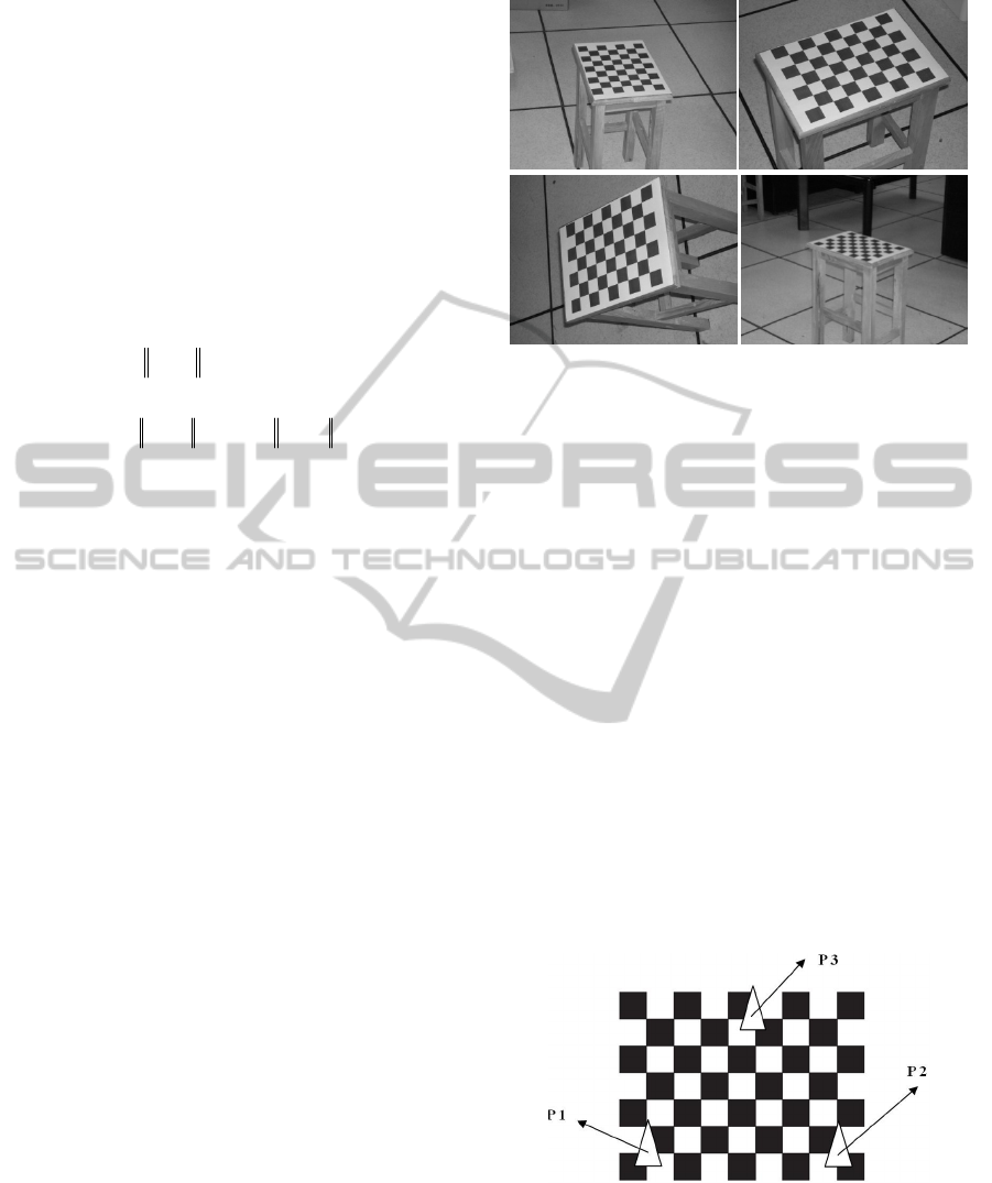
2000). As can be observed in Figure 1 below, four

images of the chessboard pattern were taken by a

Nikon COOL-PIX 4100 digital camera in an indoor

office. All the images have the resolution of

1600×1200 (in pixel). From each image, we can

extract 48 (6 rows×8 columns) corner points from

the grids. For the four images in the tests, the camera

was placed at different positions with different

orientations so as to make the proposed algorithm

work in different situations.

Figure 1: Images of chessboard pattern, from upper left to

lower right numbered 1,2,3,4.

Afterwards, the camera was calibrated from the

chessboard images (Zhang, 2000). As a result, both

the camera intrinsic and exterior parameters,

including the rotation matrix and translation vector,

were calculated. In the experiment, the camera

calibration matrix was calculated as follows

⎥

⎦

⎤

⎢

⎣

⎡

100

8.6762.41690

1.87405.4175

From the computed camera exterior parameters,

we calculate the normal of chessboard plane in the

camera coordinate system from each image, which is

the third column vector of the rotation matrix. The

3D coordinates of the control points were computed

from the rotation matrix and the translation vector,

from which the distances were calculated. They

were then acted as the ground truth data to validate

the proposed algorithm.

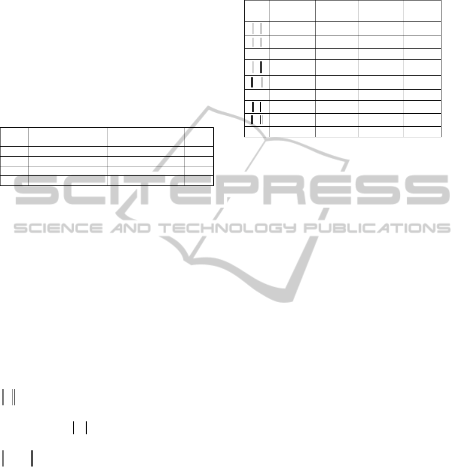
Figure 2: Three control points selected from the grids of

the chessboard pattern.

Three control points (see the points marked by

triangles and numbered P1, P2, and P3 in Figure 2)

were chosen from a number of forty-eight (6 rows×8

columns) corner points on the chessboard. Hence,

VISAPP 2011 - International Conference on Computer Vision Theory and Applications

122

the support plane coincides with the chessboard

plane. From the three control points, we derived

three length ratios and three known angles using Eq.

(4)~Eq. (6), which were then acted as the basic

geometric constraints to compute the plane normal

from each of the chessboard pattern image by using

the proposed algorithm. In the experiment, we

partitioned the Gaussian hemisphere into 400×200

cells for the searching algorithm, with each cell

representing a unit normal.

Table 1: Computation results for the normal of the support

plane (chessboard plane).

Computed Normal Actual Normal

Err

(in

)

Img1

0.078 -0.823 -0.562 0.076 -0.825 -0.560 0.20

Img2

0.034 -0.634 -0.773 0.030 -0.631 -0.776 0.33

Img3

-0.700 -0.134 -0.701 -0.697 -0.133 -0.705 0.26

Img4

0.029 -0.935 -0.354 0.027 -0.934 -0.356 0.20

Table 1 above presents the normal computation

results, where the second column is for computed

normal with the proposed algorithm, and the third

for the actual normal, or the ground truth normal

from the camera calibration results. The angle

between the estimated and actual normal reflect the

computation errors, which are represented in the

fourth column (unit in degree). It can be observed

that all error angles are less than 0.35 degrees, which

show that the proposed algorithm is accurate.

Afterwards, distances of the three control points

to the camera center were computed by homography

decomposition based on the calculated normal. The

results are presented in Table 2 below. Also, the

ground truth distances were derived from the camera

calibration results, to which the computed distances

were compared. As can be observed in Table 2,

()

3,2,1

=iP

is the computed Euclidean distance of

the i

control point to the camera, with the proposed

algorithm, while

()

3,2,1=iP

for the ground truth

distance. The Euclidean distance between them,

()

3,2,1

=− iPP

, defines the computation error. As

shown in Table 2, the distance computation errors

are very small. For example, for all the four images,

the computation errors for all the three points are

less than 0.8cm, and the average computation error

is 0.41 cm, within about 1.0~2.0m camera-to-plane

distances. The results demonstrate that the algorithm

is accurate and practical.

Table 2: Computed distances between the control points

and the camera (unit in cm).

Img1 Img2 Img3 Img4

164.3 109.3 114.0 199.8

163.6 109.0 114.5 199.9

Err

0.7 0.3 0.5 0.1

160.6 120.4 113.1 204.7

159.8 120.2 113.6 204.6

Err

0.8 0.2 0.6 0.1

176.6 114.8 126.1 216.9

175.8 114.5 126.5 216.9

Err

0.8 0.3 0.5 0

The multiple solutions of P3P problem was also

studied and illustrated with the proposed algorithm,

which is shown in Figure 3. Actually, multiple

solutions to P3P correspond to multiple support

planes. If a P3P problem has multiple solutions, the

algorithm may find a solution that is different from

the ground truth normal, because it only searches for

the maximum likelihood. As shown in Figure 3, the

likelihood map was generated by computing the

likelihood for each sampled normal on Gaussian

hemisphere using Eq. (13). In the likelihood map,

the image intensity represents the likelihood, with

darker intensity representing higher likelihood. And

the maximum likelihood was then searched

throughout the likelihood map, with the computed

plane normal

[

]

454.0888.0070.0 −−

. The

corresponding position in the likelihood map is

marked by a diamond (

◇

) (see Figure 3(b)). And the

actual normal, also the ground truth normal is

[

]

590.0802.0092.0 −−

, with the position in

the likelihood map marked by a cross (+) (see Figure

3(b)). Figure 3(c) shows the positions of thirty

normal directions, which yield the highest

likelihoods. They are located in two different areas,

with two local maxima in the likelihood map (see

Figure 3(c)), which means that it has two solutions

to the given P3P problem. The calculated normal is

located in the right part, while the actual normal in

the left (see Figure 3(c)). This is consistent with the

conclusion that P3P gives two solutions most of the

time (Wolfe et al., 1991). The results clearly

demonstrate that the proposed algorithm can be used

to study and classify the multiple solutions (two

solutions in this case) to P3P problem.

PERSPECTIVE-THREE-POINT (P3P) BY DETERMINING THE SUPPORT PLANE

123

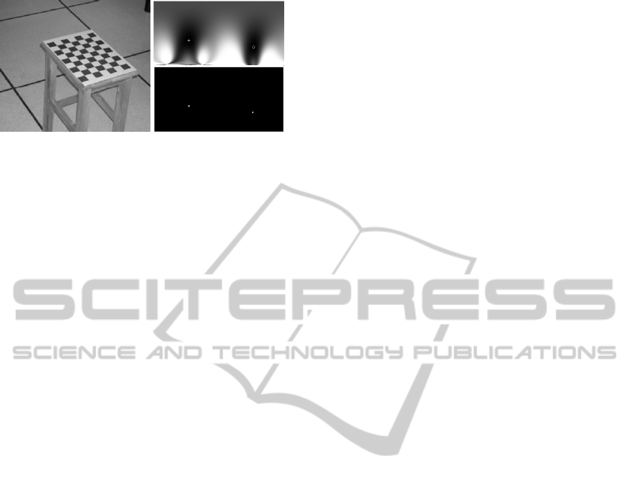
Figure 3: Illustration of two solutions to P3P: a) Left:

Original image; b) Upper right: likelihood map with

positions of the actual and computed normal marked by +

and ◇, respectively; c) Lower right: positions of the 30

normal directions with the highest likelihoods.

5 CONCLUSIONS

This paper has presented a new algorithm to solve

P3P problem by determining the support plane.

Plane normal computation is formulated as finding

the maximum likelihood on Gaussian hemisphere.

With the determined support plane, the P3P problem

can be solved by homography decomposition. The

algorithm has been tested by using actual images

with good results for plane normal and for distance

computation reported. It was also applied to study

and classify the multiple solutions to P3P problem.

This algorithm not only suggests a new approach to

P3P but also complements existing P3P researches.

Moreover, the proposed model is expected to help

solve other PnP (n=4, 5) problems and classify the

multiple solutions.

ACKNOWLEDGEMENTS

The work presented in this paper was sponsored by a

research grant from the Grant-In-Aid Scientific

Research Project (No. P10049) of the Japan Society

for the Promotion of Science (JSPS), Japan, and a

research grant (No. L2010060) of the Department of

Education, Liaoning Province, China.

REFERENCES

Fischler, M., and Bolles, R. (1981). Random sample

consensus, Communications of the ACM, Vol. 24, No.

6, pp.381-395

Gao, X., Hou, X., Tang, J., Cheng, H. (2003). Complete

solution classification for the perspective-three-point

problem, IEEE Transaction on Pattern Analysis and

Machine Intelligence, Vol. 25, No. 8, pp. 930-943

Hartley, R., and Zisserman, A. (2000). Multiple view

geometry in computer vision, Cambridge, UK:

Cambridge University Press, 2nd Edition.

Hu, Z., and Matsuyama, T. (2010). A generalized

computation model for plane normal recovery by

searching on Gaussian hemisphere, the Third

International Conference on Computer and Electricity

(ICCEE 2010), pp.145-149

Liebowitz, D., and Zisserman, A. (1998). Metric

rectification for perspective images of planes,

Proceedings of the IEEE Conference on Computer

Vision and Pattern Recognition, pp.482-488

Moreno-Noguer, F., Lepetit, V., and Fua, P. (2007).

Accurate non-iterative O(n) solution to the PnP

problem. IEEE 11th International Conference on

Computer Vision, pp. 1–8

Vigueras, F., Hern´andez, A., and Maldonado, I. (2009).

Iterative linear solution of the perspective-n-point

problem using unbiased statistics, Eighth Mexican

International Conference on Artificial Intelligence,

Guanajuato, Mexico, pp.59-64

Wolfe, W., Mathis, D., Sklair, C., Magee, M. (1991). The

perspective view of 3 Points, IEEE Transaction on

Pattern Analysis and Machine Intelligence, Vol. 13,

No. 1, pp.66-73

Wu, Y., Hu, Z. (2006). PnP problem revisited. Journal of

Mathematical Imaging and Vision, Vol. 24, No. 1, pp.

131-141

Zhang, C., Hu, Z. (2006). Why is the danger cylinder

dangerous in the P3P problem? Acta Automatiica

Sinica, Vol. 32, No. 4, pp.504-511

Zhang, Z. (2000). A flexible new technique for camera

calibration, IEEE Transaction on Pattern Analysis and

Machine Intelligence, Vol.22, No. 11, pp.1330-1334

VISAPP 2011 - International Conference on Computer Vision Theory and Applications

124