TEMPORAL POST-PROCESSING METHOD

FOR AUTOMATICALLY GENERATED DEPTH MAPS

Sergey Matyunin, Dmitriy Vatolin

Graphics & Media Lab, Moscow State University, Leninskiye Gory, Moscow, Russian Federation

Maxim Smirnov

YUVsoft Corp, Moscow, Russian Federation

Keywords:

Depth map, Filtering, Temporal post-processing, 3D video.

Abstract:

Methods of automatic depth maps estimation are frequently used for 3D content creation. Such depth maps

often contains errors. Depth ﬁltering is used to decrease the noticeability of the errors during visualization. In

this paper, we propose a method of temporal post-processing for automatically generated depth maps. Filtering

is performed using color and motion information from the source video. A comparison of the results with test

ground-truth sequences using the BI-PSNR metric is presented.

1 INTRODUCTION

Accurate and reliable depth information plays an im-

portant role in 3D video creation and processing. Cre-

ating a depth map for a conventional 2D video is a

laborious process, so methods of automatic genera-

tion are under development. One of the promising

approaches is depth reconstruction using object mo-

tion (Kim et al., 2007). In (Saxena et al., 2005), the

authors propose a method of spatial structure analysis

based on neural networks and machine learning.

Estimation of depth on the basis of stereo video

(Ogale and Aloimonos, 2005) can be used for parallax

tuning and nonlinear editing of 3D content.

The problem of deﬁnite depth reconstruction with-

out additional information is generally unsolvable.

For automatic depth reconstruction, methods that are

based on local criteria minimization can be applied.

This approach, however, leads to errors in the depth

map. Such depth maps cannot be used for 3D image

creation owing to temporal instability and errors. A

speciﬁc type of preprocessing is required to increase

the temporal and spatial stability of the results. This

paper proposes such a method of depth map process-

ing using color and motion information.

2 RELATED WORK

Depth processing is often used to decrease the notice-

ability of depth map errors during visualization. Mod-

iﬁed forms of Gaussian blur are applied in occlusion

areas (Lee and Ho, 2009). In (Tam and Zhang, 2004),

the authors propose asymmetric blurring: the ﬁlter

length is larger in the vertical direction than in the hor-

izontal direction. They also propose changing the size

of the symmetric smoothing ﬁlter depending on the

local values in the depth maps. An edge-dependent

depth ﬁlter was proposed in (Chen et al., 2005). To

increase the quality of the results, edge direction is

taken into account.

The above-mentioned approaches only use data

from the current frame, and they only use a portion

of the color information from the source video (for

example, only edges location).

A method of spatial and temporal enhancement

for depth maps captured by depth sensors was pro-

posed in (Kim et al., 2010). Motion information is

used to minimize depth ﬂickering on stationary ob-

jects. This approach only considers the presence of

the motion rather than the magnitude of the motion.

In (Zhang et al., 2009), the authors propose a

method of reducing temporal instability by solving

the energy minimization problem for several consec-

utive frames using graph cut and belief propagation.

Another approach to depth map post-processing pro-

Matyunin S., Vatolin D. and Smirnov M..

TEMPORAL POST-PROCESSING METHOD FOR AUTOMATICALLY GENERATED DEPTH MAPS.

DOI: 10.5220/0003318800330038

In Proceedings of the International Conference on Imaging Theory and Applications and International Conference on Information Visualization Theory

and Applications (IMAGAPP-2011), pages 33-38

ISBN: 978-989-8425-46-1

 2011 SCITEPRESS (Science and Technology Publications, Lda.)

posed in (Zhang et al., 2008) is iterative reﬁnement.

For each frame, the algorithm reﬁnes the depth maps

of neighboring frames. The reﬁnement procedure

is also reduced to the energy minimization problem.

Such approaches produce good results, but owing to

computational complexity, they require a long time

to process the entire video (several minutes for each

frame).

The proposed approach uses several neighboring

frames to reﬁne the depth map. Filtering is performed

by taking into account the intensity (color) similarity

of pixels and the spatial distance. The algorithm takes

information about object motion into account using

motion compensation.

3 PROPOSED METHOD

For the ﬁltering of the current depth map D

the algorithm uses the neighboring source frames

n−m

, . . . , I

n+m

and the depth maps D

n−m

, . . . , D

n+m

(x, y) denotes the intensity (or color) of pixel (x, y)

in frame i. I

(x, y) is either a three-vector for a color

image or a scalar for a grayscale image. The proposed

method consists of four steps:

1. Motion estimation between the current frame

and neighboring frames I

n−m

, . . . , I

n−1

n+1

, . . . , I

n+m

, where m > 0 is a parameter.

The result of this stage is a ﬁeld of motion

vectors MV

(x, y) = (u

(x, y), v

(x, y)). We deﬁne

(x, y) ≡ (0, 0).

2. Computation of the conﬁdence metric C

(x, y) for

the resultant motion vectors MV

(x, y). Here,

(x, y) ∈ [0, 1]. C

(x, y) quantiﬁes the estimation

quality for motion vector MV

(x, y).

3. Motion compensation for the depth maps and the

source frames:

(x, y) = I

(x +u

(x, y), y +v

(x, y)),

(x, y) = D

(x +u

(x, y), y +v

(x, y)),

where D

denotes the motion-compensated

depth maps, and I

denotes the motion-

compensated source frames.

4. Depth map ﬁltering using the computed D

, C

and I

values.

3.1 Motion Estimation

We used a block matching motion estimation algo-

rithm based on the algorithm described in (Simonyan

cones teddy sawtooth bull venus

Sequence

BI−PSNR, dB

Before filtering

After filtering

Figure 1: Results of the objective quality assessment. Depth

maps were compared with ground truth depth before and

after ﬁltering. The comparison was performed using the

Brightness Independent PSNR metric.

et al., 2008b). The algorithm uses macroblocks of size

16×16, 8 ×8 and 4×4 with adaptive partitioning cri-

teria. Motion estimation is performed with quarter-

pixel precision. Both luminance and chroma planes

are considered.

3.2 Conﬁdence Metric

The motion estimation algorithm often produces

wrong motion vectors, especially in the occlusion ar-

eas. Wrong motion estimation leads to artifacts. To

reduce the inﬂuence of outliers we introduce conﬁ-

dence metric C for motion vectors. The metric is

based on that described in (Simonyan et al., 2008a).

C = (1 − α)∗C

SAD

+ α ∗C

where C

SAD

responds to the motion-compensated in-

terframe difference and C

responds to the spa-

tial smoothness of motion vectors ﬁeld in the spa-

tial neighborhood of the current block. α ∈ [0, 1] de-

scribes the smoothness of the current block.

3.3 Filtering

The ﬁlter consists of two stages. The ﬁrst stage is tem-

poral median ﬁltering. Median ﬁltering is often used

to eliminate sharp discontinuities in the time domain.

We apply ﬁltering to the motion compensated frames

to make our approach usable for the video sequences

with fast motion. In order to reduce the inﬂuence of

the errors of motion compensation we consider only

those pixels (x, y) from the neighboring depth maps

which have a good conﬁdence metric value and

small interframe difference |I

(x, y) −I

(x, y)|:

IMAGAPP 2011 - International Conference on Imaging Theory and Applications

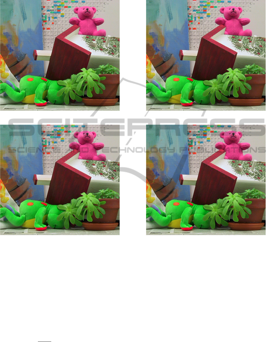
a) Source frame. b) Ground truth.

c) Estimated depth map. d) Filtered depth map.

Figure 2: Sequence ”Teddy”.

med

(x, y) = median

{

(x, y)



i ∈ [n −m, . .. , n +m],C

(x, y) > T h

(x, y) − I

(x, y)| < T h

SAD

}

(1)

Thresholds T h

and T h

SAD

depend on the noise

level of the source video. The second stage of the

ﬁltering is temporal smoothing. We average the depth

over the spatio-temporal neighborhood of the current

pixel with weights ω(t, x, y, x

′

, y

′

smooth

(x, y) =

k(x, y)

n+m

∑

t=n−m

∑

′

)∈σ(x,y)

(ω(t, x, y, x

′

, y

′

)·

·D

med

′

, y

′

)),

(2)

where k(x, y) is a normalization term:

k(x, y) =

n+m

∑

t=n−m

∑

′

)∈σ(x,y)

ω(t, x, y, x

′

, y

′

). (3)

σ(x, y) denotes the small spatial neighborhood of

pixel (x, y). The size of σ(x, y) is chosen as a trade-

off between computation speed and processing qual-

ity. Smaller σ(x, y) produces worse results for noisy

video.

Previous fully processed depth D

smooth

can be

used instead of D

med

in (2). This approach yields a

more stable result, but at the expense of quality of

processing for small details.

Weighting function ω is given by

ω(t, x, y, x

′

, y

′

) = f (t, x

′

, y

′

)·C

′

, y

′

)· g(x −x

′

, y − y

′

TEMPORAL POST-PROCESSING METHOD FOR AUTOMATICALLY GENERATED DEPTH MAPS

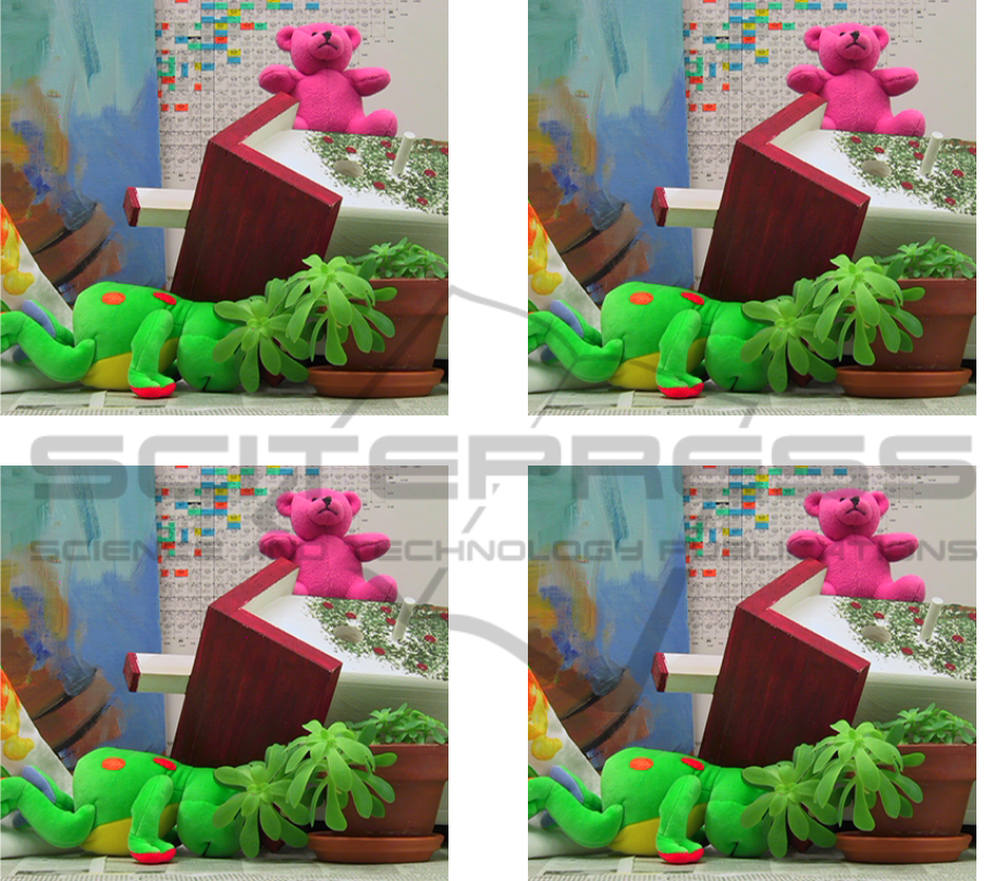
a) Source frame. b) Ground truth.

c) Estimated depth map. d) Filtered depth map.

Figure 3: Sequence ”Cones”.

where function f (t, x

′

, y

′

) denotes the quadratic func-

tion of the motion-compensated inter-frame differ-

ence |I

′

, y

′

) − I

′

, y

′

)|; C

′

, y

′

) is the conﬁ-

dence metric of motion estimation of pixel (x

′

, y

′

) in

frame t; g(x, y) is a Gaussian function.

If the neighboring pixel (x

′

, y

′

) belongs to the area

with good conﬁdence and has a color similar to the

color of current pixel (x, y), then the depth of (x

′

, y)

′

has more inﬂuence on the resulting depth of pixel

(x, y). Thus, the algorithm averages the depth in

the neighborhood of each pixel using the information

about the motion-compensated interframe difference

for the source video, the conﬁdence metric for motion

vectors, and the spatial proximity.

4 RESULTS

The proposed algorithm was implemented in C as a

console application. The algorithm uses one-pass pro-

cessing, and it can be conveniently implemented in

hardware. The algorithm’s performance on an Intel

Core2Duo T6670 processor running at 2.20 GHz is

7.6 fps for 448 × 372 video resolution. A time of the

depth map estimation was not included in the mea-

surement. The most time consuming stage of the al-

gorithm is the motion estimation. Without regard for

the motion estimation, the proposed method allows to

ﬁlter the depth map in linear time with respect to the

size of the image.

IMAGAPP 2011 - International Conference on Imaging Theory and Applications

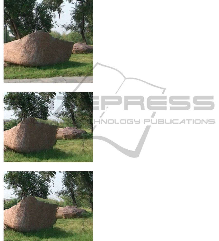
a) Original 2D image.

b) Rendered view for the estimated depth map.

c) Rendered view for the ﬁltered depth map.

Figure 4: Depth based rendered view. Segment of ”Road”

sequence. The rendered view based on the ﬁltered depth

seems more natural. The depth map was ﬁltered using the

proposed method and the cross bilateral ﬁltering. Occlu-

sions are not processed.

All the source depth maps for quality evaluation

were obtained using the depth-from-motion method

based on that described in (Ogale and Aloimonos,

2005). We used ﬁve consecutive frames for ﬁltering

(m = 2) in our experiments. m > 3 gives satisfactory

results only on the stationary video sequences because

of unreliable motion estimation for distant frames.

For an objective evaluation, the standard se-

quences ”Cones,” ”Venus,” ”Sawtooth,” ”Teddy” and

”Bull” were used (Scharstein and Szeliski, 2002;

Scharstein and Szeliski, 2003). Each data set is a

multi-baseline stereo sequence, i.e., the frames are

taken from equally-spaced viewpoints along the hori-

zontal axis. The latter allows to consider the ground-

truth disparities as the representation of the depth.

The comparison with ground truth was performed us-

ing the Brightness Independent PSNR metric (Vatolin

et al., 2009). Fig. 1 shows the results.

For a subjective evaluation, Fig. 2 depicts the

results of the algorithm for the sequence ”Teddy”.

The depth map (Fig. 2b) generated from the source

video sequence (Fig. 2a) was ﬁltered using the pro-

posed method. The ﬁltering process restored some

lost details and ﬁxed depth-estimation errors on ob-

ject boundaries (Fig. 2d). Fig. 3 shows the results for

the sequence ”Cones”.

One of the main drawbacks of the proposed algo-

rithm is producing undesirable texture on some depth

maps. This problem can be solved using spatial ﬁlter-

ing. Cross bilateral post-processing (Petschnigg et al.,

2004) gives rather good results (Fig. 4). The proposed

method allowed to reduce artifacts on the resulting

rendered view and improve visual quality.

5 CONCLUSIONS

In this paper, we described a post-processing method

algorithm for depth maps that are automatically gen-

erated from video. The proposed method shows high

quality of ﬁltering, uses single-pass processing, and

doesn’t require complex calculations (e.g., energy

minimization or color segmentation). The algorithm’s

integration with a spatial post-ﬁltering can be used as

a high-performance processing method for the depth

maps.

ACKNOWLEDGEMENTS

This research was partially supported by grant num-

ber 10-01-00697-a from the Russian Foundation for

Basic Research.

TEMPORAL POST-PROCESSING METHOD FOR AUTOMATICALLY GENERATED DEPTH MAPS

REFERENCES

Chen, W.-Y., Chang, Y.-L., Lin, S.-F., Ding, L.-F., and

Chen, L.-G. (2005). Efﬁcient depth image based ren-

dering with edge dependent depth ﬁlter and interpola-

tion. IEEE International Conference on Multimedia

and Expo, 0:1314–1317.

Kim, D., Min, D., and Sohn, K. (2007). Stereoscopic video

generation method using motion analysis. In 3DTV

Conference, pages 1–4.

Kim, S.-Y., Cho, J.-H., Koschan, A., and Abidi, M. A.

(2010). Spatial and temporal enhancement of depth

images captured by a time-of-ﬂight depth sensor.

In International Conference on Pattern Recognition

(ICPR), pages 2358–2361. IEEE.

Lee, S.-B. and Ho, Y.-S. (2009). Discontinuity-adaptive

depth map ﬁltering for 3d view generation. In Pro-

ceedings of the 2nd International Conference on Im-

mersive Telecommunications, pages 1–6.

Ogale, A. S. and Aloimonos, Y. (2005). Shape and the

stereo correspondence problem. International Jour-

nal of Computer Vision, 65(3):147–162.

Petschnigg, G., Agrawala, M., Hoppe, H., Szeliski, R., Co-

hen, M., and Toyama, K. (2004). Digital photography

with ﬂash and no-ﬂash image pairs. In SIGGRAPH,

pages 664–672.

Saxena, A., Chung, S. H., and Ng, A. Y. (2005). Learn-

ing depth from single monocular images. In Advances

in Neural Information Processing Systems 18, pages

1161–1168. MIT Press.

Scharstein, D. and Szeliski, R. (2002). A taxonomy and

evaluation of dense two-frame stereo correspondence

algorithms. International Journal of Computer Vision,

47(1-3):7–42.

Scharstein, D. and Szeliski, R. (2003). High-accuracy

stereo depth maps using structured light. IEEE Com-

puter Society Conference on Computer Vision and

Pattern Recognition, 1:195.

Simonyan, K., Grishin, S., and Vatolin, D. . (2008a). Conﬁ-

dence measure for block-based motion vector ﬁeld. In

GraphiCon, pages 110–113.

Simonyan, K., Grishin, S., Vatolin, D., and Popov, D.

(2008b). Fast video super-resolution via classiﬁca-

tion. In International Conference on Image Process-

ing, pages 349–352. IEEE.

Tam, W. J. and Zhang, L. (2004). Non-uniform smoothing

of depth maps before image-based rendering. In Pro-

ceedings of Three-Dimensional TV, Video and Display

III (ITCOM’04), volume 5599, pages 173–183.

Vatolin, D., Noskov, A., and Grishin, S. (2009).

MSU Brightness Independent PSNR (BI-PSNR).

http://compression.ru/video/quality measure/metric

plugins/bi-psnr en.htm.

Zhang, G., Jia, J., Wong, T.-T., and Bao, H. (2008). Re-

covering consistent video depth maps via bundle op-

timization. In IEEE Conference on Computer Vision

and Pattern Recognition, pages 1 – 8.

Zhang, G., Jia, J., Wong, T.-T., and Bao, H. (2009). Con-

sistent depth maps recovery from a video sequence.

IEEE Transactions on Pattern Analysis and Machine

Intelligence, 31(6):974–988.

IMAGAPP 2011 - International Conference on Imaging Theory and Applications