BAG OF WORDS FOR LARGE SCALE OBJECT RECOGNITION
Properties and Benchmark
Mohamed Aly
1
, Mario Munich
2
and Pietro Perona
1
1
Computational Vision Lab, Caltech, Pasadena, CA, U.S.A.
2
Evolution Robotics, Pasadena, CA, U.S.A.
Keywords:
Image search, Image retrieval, Bag of words, Inverted file, Min hash, Benchmark, Object recognition.
Abstract:
Object Recognition in a large scale collection of images has become an important application of widespread
use. In this setting, the goal is to find the matching image in the collection given a probe image containing the
same object. In this work we explore the different possible parameters of the bag of words (BoW) approach
in terms of their recognition performance and computational cost. We make the following contributions: 1)
we provide a comprehensive benchmark of the two leading methods for BoW: inverted file and min-hash; and
2) we explore the effect of the different parameters on their recognition performance and run time, using four
diverse real world datasets.
1 INTRODUCTION
Object recognition in a large scale collection of im-
ages has become an important problem of widespread
use. There are currently several smart phone applica-
tions that allow the user to take a photo and search
a database of stored images e.g. Google Goggles
1
and Barnes and Noble
2
apps. These image collections
typically include images of book covers, CD/DVD
covers, retail products, and buildings and landmark
images. Database sizes vary from 10
5
to 10
7
images,
and they can conceivably reach billions of images.
The ultimate goal is to identify the database image
containing the object depicted in a probe image, e.g.
an image of a book cover from a different view point
and scale. The correct image can then be presented
to the user, together with some revenue generating in-
formation, e.g. sponsor ads or referral links.
It has been shown that bag of words (BoW) ap-
proach provides several advantages (Philbin et al.,
2007; Chum et al., 2007b; J
´
egou et al., 2008; Aly
et al., 2009b; Chum et al., 2009; Nister and Stewe-
nius, 2006) over the traditional approach of match-
ing local features(Lowe, 2004): acceptable recogni-
tion performance, faster run time, and reduced stor-
age. They have been used in image retrieval settings
(Philbin et al., 2007; J
´
egou et al., 2008; Nister and
1
http://tinyurl.com/yla655ztinyurl.com/yla655z
2
http://tinyurl.com/mstn5btinyurl.com/mstn5b
Stewenius, 2006), near duplicate detection (Chum
et al., 2007a; Chum et al., 2008), and image cluster-
ing (Aly et al., 2009b). The two leading methods for
BoW are Inverted File (Zobel and Moffat, 2006) and
Min-Hash (Broder et al., 1997; Broder et al., 2000).
The former is an efficient exact search method to find
nearest neighbors, while the latter is an efficient ap-
proximation. Both methods have a lot of parameters
and settings that represent trade off between run time
and performance. In this work we explore those pa-
rameters to assess their effect on the recognition per-
formance and run time.
We make the following contributions:
1. We provide a comprehensive benchmark of the
two leading methods for BoW: Inverted File (IF)
and Min-Hash (MH) in the object recognition set-
ting
2. We explore the effect of the different parame-
ters of these methods on the recognition perfor-
mance and the run time, using four real world
datasets with diverse statistics. In particular, we
consider the following: IF parameters, MH pa-
rameters, dictionary size, dictionary type, and ge-
ometric consistency check.
299
Aly M., Munich M. and Perona P..
BAG OF WORDS FOR LARGE SCALE OBJECT RECOGNITION - Properties and Benchmark.
DOI: 10.5220/0003311402990306
In Proceedings of the International Conference on Computer Vision Theory and Applications (VISAPP-2011), pages 299-306
ISBN: 978-989-8425-47-8
Copyright
c
 2011 SCITEPRESS (Science and Technology Publications, Lda.)

2 METHODS OVERVIEW
In this work we consider the two leading methods
of the BoW approach: Inverted File and Min-Hash.
They represent different levels of approximation, and
differ in how they store the images histograms and in
how they perform the nearest neighbor search. The
basic BoW idea is described in Algorithm 1. We only
provide a brief description of the methods for brevity.
Algorithm 1: Basic Bag of Words Matching Algorithm.
1. Extract features {f
i j
}
j
from every database image i
2. Build a dictionary of “visual words”
3. For database images:
(a) find the corresponding visual word of every feature
(b) Build a histogram of visual words
4. Build a data structure D based on these histograms
5. Given a probe image q, extract its local features and
compute its histogram of visual words
6. Search the data structure D for “nearest neighbors”
7. Every nearest neighbor votes for the database image i it
comes from, accumulating to its score s
i
8. Sort the database images based on their score s
i
, and
report the top scoring image as the matching image
9. (Optional) Post-process the sorted list of images to en-
force some geometric consistency and obtain a final list
of sorted images s
0
i
. The geometric consistency check is
done using a RANSAC algorithm to fit an affine trans-
formation between the query image q and the database
image i.
1. Inverted File (IF). The images histograms are
stored in such a way to provide faster search time
(Baeza-Yates and Ribeiro-Neto, 1999; Zobel and
Moffat, 2006). The idea is to store for every vi-
sual word the list of images that contain it. At
run time, only images with overlapping words are
processed, and this saves a lot of time and pro-
vides exact search results.
2. Min-Hash (MH). The histograms are binarized
(counts are ignored), and each image is repre-
sented as a “set” of visual words {b
i
}
i
. Then,
a number of locality sensitive hash functions
(Broder et al., 1997; Broder, 1997; Broder et al.,
2000; Chum et al., 2007a) are extracted from
the database binary histograms {b
i
}
i
, and are ar-
ranged in a set of tables. . The hash function is
defined as h(b) = min π(b) where π is a random
permutation of the numbers {1, ..., W} where W
is the number of words in the dictionary. At run
time, images that have the same hash value are
ranked according to the amount of overlap of their
binary histograms.
3 EVALUATION DETAILS
3.1 Datasets
We use the same setup as in (Aly et al., 2011). Specif-
ically, we have two kinds of datasets:
1. Distractors: images that constitute the bulk of the
database to be searched. In the actual setting, this
would include all the objects of interest e.g. book
covers, ... etc.
2. Probe: labeled images, two types per object:
(a) Model Image: the ground truth image to be
retrieved for that object
(b) Probe Images: “distorted” images for each ob-
ject that are used for querying the database,
representing the object in the model image
from different view points, lighting conditions,
scales, ... etc.
Figure 1: Example distractor images. Each row depicts a
different set: D1, D2, D3, and D4, respectively, see sec.
3.1.
Distractor Sets
• D1: Caltech-Covers. A set of ˜ 100K images of
CD/DVD covers used in (Aly et al., 2009a).
• D2: Flickr-Buildings. A set of ˜1M
images of buildings collected from
http://flickr.comflickr.com
• D3: Image-net. A set of ˜400K images of “ob-
jects” collected from http://image-net.orgimage-
net.org, specifically images under synsets: instru-
ment, furniture, and tools.
• D4: Flickr-Geo. A set of ˜1M geo-tagged images
collected from http://flickr.comflickr.com
Figure 1 shows some examples of images from these
distractor sets.
Probe Sets
• P1: CD Covers. A set of 5×97=485 images of
CD/DVD covers.
• P2: Pasadena Buildings. A set of 6×125=750
images of buildings around Pasadena, CA from
(Aly et al., 2009a).
VISAPP 2011 - International Conference on Computer Vision Theory and Applications
300

Figure 2: Example probe images. Each row depicts a differ-
ent set: P1, P2, P3, and P4, respectively. Each row shows
two model images and 2 or 3 of its probe images, see sec.
3.1.
Table 1: Probe Sets Properties and Evaluation Scenarios.
Probe Sets
total #model #probe
P1 485 97 388
P2 750 125 525
P3 720 80 640
P4 957 233 724
Evaluation Scenarios
Scenario Distractor Probe
1 D1 P1
2 D2 P2
3 D3 P3
4 D4 P4
• P3: ALOI. A set of 9×80=640 3D objects
images from the ALOI collection (Geusebroek
et al., 2005) with different illuminations and view
points.
• P4: INRIA Holidays. a set of 957 images, which
forms a subset of images from (J
´
egou et al., 2008),
with groups of at least 3 images.
Figure 2 shows some examples of images from these
distractor sets. Table 1 summarizes the properties of
these probe sets.
3.2 Setup
We used four different evaluation scenarios, where in
each we use a specific distractor/probe set pair. Ta-
ble 1 lists the scenarios used. Evaluation was done
by increasing the size of the dataset from 100, 1k,
10k, 50k, 100k, and 400K. For each such size, we
include all the model images to the specified num-
ber of distractor images e.g. for 1k images, we have
1000 images from the distractor set in addition to all
images in the probe set. Performance is measured as
the percentage of probe images correctly matched to
their ground truth model image i.e. whether the cor-
rect model image is the first ranked image returned.
We want to emphasize the difference between the
setup used here and the setup used in other “image
retrieval”-like papers (J
´
egou et al., 2008; Chum et al.,
2008; Philbin et al., 2007). In our setup, we have
only ONE correct ground truth image to be retrieved
and several probe images, while in the other setting
there are a number of images that are considered cor-
rect retrievals. This is motivated by the application
under consideration, for example, identifying the cor-
rect identity of the query image of a DVD cover.
We use SIFT (Lowe, 2004) feature descriptors
with hessian affine (Mikolajczyk and Schmid, 2004)
feature detectors. We used the binary available from
http://tinyurl.com/vgg123tinyurl.com/vgg123. Each
scenario has its own sets of dictionaries, which are
built using a random subset of 100k images of the
corresponding distractor set. The probe sets were
not included in the dictionary generation to avoid bi-
asing the results. All experiments were performed
on machines with Intel dual Quad-Core Xeon E5420
2.5GHz processor and 32GB of RAM. We imple-
mented all the algorithms using Matlab and Mex/C++
scripts
3
.
4 METHODS PARAMETERS
4.1 Inverted File Parameters
In the Inverted File method, we can use different com-
binations of histogram weighting, normalizations,
and distance functions:
Weighting:
1. none: use the raw histogram
2. binary: binarize the histogram i.e. just record
whether the image has the visual word or not
3. tf-idf: weight the counts in such a way to decrease
the influence of more common words and increase
the influence of more distinctive words
Normalizations: how to normalize the histograms
1. l
1
: normalize so that
∑
i
|h
i
| = 1
2. l
2
: normalize so that
∑
i
h
2
i
= 1
Distance:
1. l
1
: use the sum of absolute differences i.e.
d
l1
(h, g) =
∑
i
|h
i
− g
i
|
2. l
2
: use the sum of squared differences i.e.
d
l2
(h, g) =
∑
i
(h
i
− g
i
)
2
3. cos: use the dot product i.e. d
cos
(h, g) = 2 −
∑
i
h
i
×g
i
. Note that for l
2
-normalized histograms,
this is equivalent to l
2
distance since ||h||
2
=
||g||
2
= 1 and d
l2
= ||h − g||
2
2
= ||h||
2
2
+ ||g||
2
2
−
2
∑
i
h
i
g
i
= 2 − 2
∑
i
h
i
g
i
.
We consider the following five combinations
{weighting, normalization, distance}:
• {tf-idf, l
2
, cos}: This is the standard way of
computing nearest neighbors in IF (Philbin et al.,
2007; Philbin et al., 2008).
3
http://vision.caltech.edu/malaa/software/research/image-
search/ http://vision.caltech.edu/malaa/software/research/image-search/
BAG OF WORDS FOR LARGE SCALE OBJECT RECOGNITION - Properties and Benchmark
301

10
2
10
4
10
6
20
40
60
80
100
Scenario 1
Number of Images
Recognition Performance
10
2
10
4
10
6
10
−1
10
0
10
1
Scenario 1
Number of Images
Search time (sec/image)
ivf−none−l1−l1
ivf−none−l2−l2
ivf−tfidf−l2−cos
ivf−bin−l1−l1
ivf−bin−l2−l2
10
2
10
4
10
6
20
40
60
80
100
Scenario 2
Number of Images
Recognition Performance
10
2
10
4
10
6
10
−1
10
0
10
1
Scenario 2
Number of Images
Search time (sec/image)
10
2
10
4
10
6
20
40
60
80
100
Scenario 3
Number of Images
Recognition Performance
10
2
10
4
10
6
10
−1
10
0
10
1
Scenario 3
Number of Images
Search time (sec/image)
10
2
10
4
10
6
20
40
60
80
100
Scenario 4
Number of Images
Recognition Performance
10
2
10
4
10
6
10
−1
10
0
10
1
Scenario 4
Number of Images
Search time (sec/image)
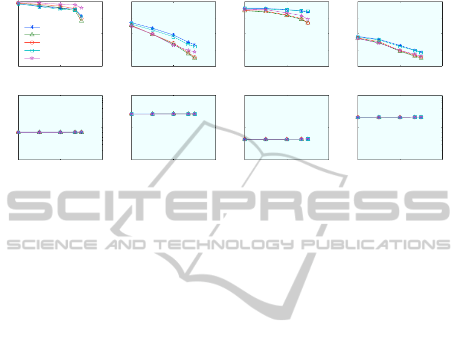
Figure 3: Effect of Inverted File (IF) Parameters. Results for different weightings, normalizations, and distance functions
using dictionaries of 1M words. Recognition performance is measured before any geometric checks, and time represents
visual words computation and IF search. See sec. 4.1.
• {bin, l
2
, l
2
}, {bin, l
1
, l
1
}: The first was shown to
work well with larger dictionaries in (J
´
egou et al.,
2009). The second is a novel one using l
1
dis-
tance.
• {none, l
1
, l
1
}, {none, l
2
, l
2
}: These use the l
1
&
l
2
distance on the raw histograms.
Figure 3 shows results for these different combi-
nations on a dictionary of 1 million visual words
computed using the Approximate K-Means (AKM)
(Philbin et al., 2007) method. We first note that the
run time is similar for all methods. This run time in-
cludes both the time to compute the visual words of
the features and the time to search the IF. We note that
using the standard combination {tf-idf, l
2
, cos} is gen-
erally inferior to the rest, and quite similar to {none,
l
2
, l
2
} i.e. leaving out the tf-idf weighting does not af-
fect performance. We also confirm that using binary
histograms yields better performance. We also note
that using binary histograms outperforms the standard
combination, as shown in (J
´
egou et al., 2009).
Finally, we note that using the l
1
distance is gen-
erally significantly superior to using cos distance, es-
pecially with raw (as reported in (Nister and Stewe-
nius, 2006)) but with binary histograms as well. This
might be explained in that it gathers more informa-
tion, since in the d
cos
, whenever a word is missing
from one image, it is left out of the calculations re-
gardless of whether the other image includes it or not.
On the other hand, with l
1
distance, this information
is taken into account.
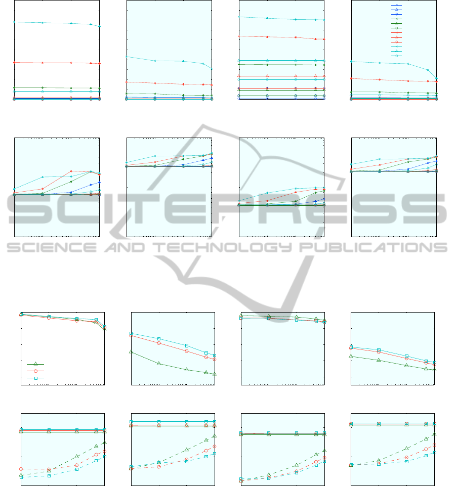
4.2 Min-Hash Parameters
Min-Hash has two parameters: (a) Number of hash
functions per table H, and (b) Number of hash tables
T . We tried different sizes for hash functions: 1, 2,
and 3 and different numbers of tables: 1, 5, 25, and
100. Figure 4 show results for these different set-
tings. Performance is measured after the geometric
consistency check, since performance beforehand is
significantly worse. Likewise, time represents the to-
tal processing time: visual words computation, MH
search and RANSAC. It is clear that using more hash
tables and less hash functions yields better results, in
particular, using 100 tables with 1 function each gives
the best overall performance, while the search time is
not significantly larger than using 25 tables.
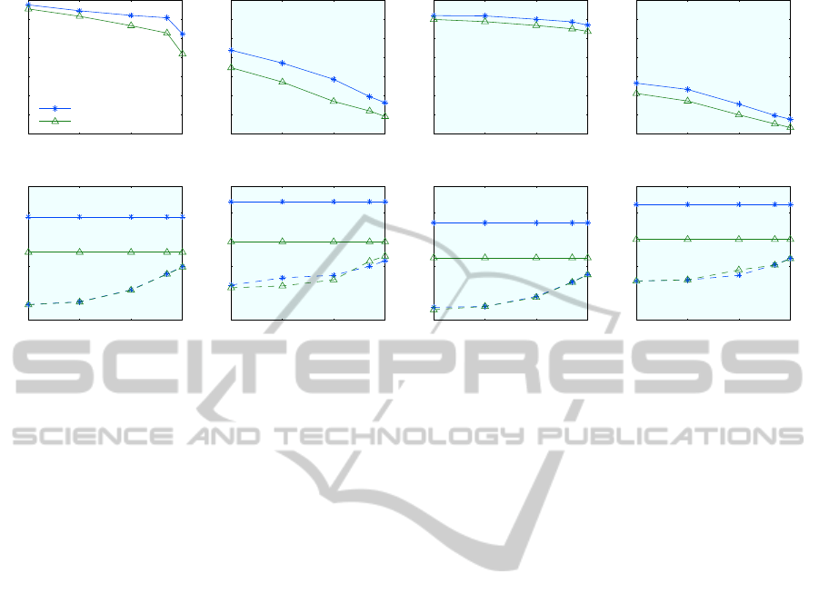
4.3 Dictionary Size
The number of visual words in the dictionary affects
greatly the recognition performance and run time of
the BoW approach. It has been shown that using
larger dictionaries, in the order of hundreds of thou-
sands, improves performance and reduces search time
in the inverted file. Dictionaries were generated us-
ing the Approximate K-Means (AKM) (Philbin et al.,
2007) method using random Kd-trees (Arya et al.,
1998) to perform an approximate nearest neighbor
search. Figure 5 shows results for using {none, l
1
,
l
1
} combination with dictionaries of sizes 10K, 100K,
and 1M visual words. We note that increasing the dic-
tionary size generally increases the recognition per-
formance, specially with harder scenarios like 2 and
VISAPP 2011 - International Conference on Computer Vision Theory and Applications
302

10
2
10
3
10
4
10
5
0
10
20
30
40
50
60
70
80
90
100
Scenario 1
Number of Images
Recognition Performance
10
2
10
3
10
4
10
5
10
−1
10
0
10
1
Scenario 1
Number of Images
Search time (sec/image)
10
2
10
3
10
4
10
5
0
10
20
30
40
50
60
70
80
90
100
Scenario 2
Number of Images
Recognition Performance
10
2
10
3
10
4
10
5
10
−1
10
0
10
1
Scenario 2
Number of Images
Search time (sec/image)
10
2
10
3
10
4
10
5
0
10
20
30
40
50
60
70
80
90
100
Scenario 3
Number of Images
Recognition Performance
10
2
10
3
10
4
10
5
10
−1
10
0
10
1
Scenario 3
Number of Images
Search time (sec/image)
10
2
10
3
10
4
10
5
0
10
20
30
40
50
60
70
80
90
100
Scenario 4
Number of Images
Recognition Performance
10
2
10
3
10
4
10
5
10
−1
10
0
10
1
Scenario 4
Number of Images
Search time (sec/image)
minhash−t1−f1
minhash−t1−f2
minhash−t1−f3
minhash−t5−f1
minhash−t5−f2
minhash−t5−f3
minhash−t25−f1
minhash−t25−f2
minhash−t25−f3
minhash−t100−f1
minhash−t100−f2
minhash−t100−f3
Figure 4: Effect of Min-Hash (MH) Parameters. Results for different numbers of hash functions and hash tables using
dictionaries of 1M words. Recognition performance is measured after the geometric step, and time represents total processing
time. See sec. 4.2.
10
2
10
3
10
4
10
5
20
40
60
80
100
Scenario 1
Number of Images
Recognition Performance
10
2
10
3
10
4
10
5
10
−4
10
−2
10
0
Scenario 1
Number of Images
Search time (sec/image)
bow−akmeans−10k
bow−akmeans−100k
bow−akmeans−1M
10
2
10
3
10
4
10
5
20
40
60
80
100
Scenario 2
Number of Images
Recognition Performance
10
2
10
3
10
4
10
5
10
−4
10
−2
10
0
Scenario 2
Number of Images
Search time (sec/image)
10
2
10
3
10
4
10
5
20
40
60
80
100
Scenario 3
Number of Images
Recognition Performance
10
2
10
3
10
4
10
5
10
−4
10
−2
10
0
Scenario 3
Number of Images
Search time (sec/image)
10
2
10
3
10
4
10
5
20
40
60
80
100
Scenario 4
Number of Images
Recognition Performance
10
2
10
3
10
4
10
5
10
−4
10
−2
10
0
Scenario 4
Number of Images
Search time (sec/image)
Figure 5: Effect of dictionary size. Results for {none, l
1
, l
1
} combination with different dictionary sizes: 10K, 100K, and 1M
visual words built with AKM. In the bottom row, solid lines represent time to compute visual words, while dashed lines show
time to search the inverted file. See sec. 4.3.
4. We also note that with larger dictionaries, the
time to compute visual words for features increases
slightly (since we are using Kd-trees), however, the
time to search the IF decreases. This is intuitive since
the number of images with similar words goes down
as the number of words increases. This suggests that
using larger dictionaries is generally the way to go.
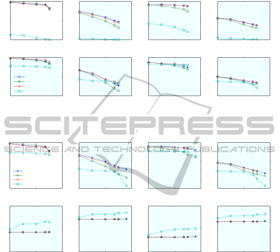
4.4 Dictionary Type
The two leading methods to compute dictionaries
with large number of words are:
BAG OF WORDS FOR LARGE SCALE OBJECT RECOGNITION - Properties and Benchmark
303

10
2
10
3
10
4
10
5
30
40
50
60
70
80
90
100
Scenario 1
Number of Images
Recognition Performance
10
2
10
3
10
4
10
5
10
−4
10
−2
10
0
Scenario 1
Number of Images
Search time (sec/image)
bow−akmeans−1M
bow−hkm−1M
10
2
10
3
10
4
10
5
30
40
50
60
70
80
90
100
Scenario 2
Number of Images
Recognition Performance
10
2
10
3
10
4
10
5
10
−4
10
−2
10
0
Scenario 2
Number of Images
Search time (sec/image)
10
2
10
3
10
4
10
5
30
40
50
60
70
80
90
100
Scenario 3
Number of Images
Recognition Performance
10
2
10
3
10
4
10
5
10
−4
10
−2
10
0
Scenario 3
Number of Images
Search time (sec/image)
10
2
10
3
10
4
10
5
30
40
50
60
70
80
90
100
Scenario 4
Number of Images
Recognition Performance
10
2
10
3
10
4
10
5
10
−4
10
−2
10
0
Scenario 4
Number of Images
Search time (sec/image)
Figure 6: Effect of dictionary type. Results for using AKM and HKM dictionaries with 1M words. In the bottom row,
solid lines represent time to compute visual words, while dashed lines show time to search the inverted file. Performance is
measured before any geometric checks. See sec. 4.4.
1. Approximate K-Means (AKM): which approx-
imates the nearest neighbor search within K-
Means using a set of randomized Kd-trees
(Philbin et al., 2007).
2. Hierarchical K-Means (HKM): which builds a
vocabulary tree by applying K-Means recursively
(Nister and Stewenius, 2006) at each node in the
tree.
Figure 6 shows results comparing these two methods
with 1M words. AKM uses 8 kd-trees with 100 back-
tracking steps, while HKM uses a tree of depth 6 with
a branching factor of 10. Recognition performance
for AKM is slightly better than HKM, however, it is at
least 10 times slower (note that the time to search the
IF is the same for both). This suggests that for time
sensitive applications, it is acceptable to use HKM at
the expense of a slight decrease in performance.
4.5 Geometric Consistency Check
After getting initial candidate matching images from
either IF or MH, there is an optional step of re-ranking
these images by using geometric consistency of corre-
sponding features. Feature matching is done crudely
using the visual words, i.e. features that have the same
visual word are considered matched. Other more ad-
vanced techniques can be used, for example (J
´
egou
et al., 2008), but here we consider the simplest ap-
proach. These feature matches are then used to fit an
affine transformation between the probe image and
the candidate images using RANSAC (Forsyth and
Ponce, 2002). The images are then sorted based on
the number of inliers. The geometric step is crucial
for MH method, and without it the performance is dis-
astrous.
For IF, it sometimes help, as in scenario 1, and
sometimes does not. We believe this depends on the
nature of the dataset. For scenario 1, the dataset
consists of CD covers with flat art, strong geomet-
ric properties, and less clutter. However, this is not
the case with the rest of the datasets, especially 2 &
4, which have buildings and other objects of interest
surrounded by a lot of clutter e.g. trees, street pave-
ments, sky, clouds, ... etc. This gives the geometric
check much harder time and makes the number of in-
liers for the true match go down by matching also to
clutter from other images. This suggests that for some
applications, we can do away with the geometric step
altogether when using IF. Note also that after the geo-
metric step MH gives performance that is comparable
to, but slightly worse than, IF.
4.6 Benchmark and Conclusions
Figure 8 shows a comparison of both MH and IF us-
ing the best parameters. For IF, we report perfor-
mance before the geometric step, as it is generally
not needed, and for MH we report performance after-
wards. We notice that IF gives superior recognition
performance and less run time, especially when using
l
1
distance function, compared to MH.
We note the following:
VISAPP 2011 - International Conference on Computer Vision Theory and Applications
304

10
2
10
4
10
6
0
50
100
Scenario 1
Number of Images
Performance (before)
10
2
10
4
10
6
0
50
100
Scenario 1
Number of Images
Performance (after)
ivf−none−l1−l1
ivf−tfidf−l2−cos
ivf−bin−l1−l1
minhash−t100−f1
10
2
10
4
10
6
0
50
100
Scenario 2
Number of Images
Performance (before)
10
2
10
4
10
6
0
50
100
Scenario 2
Number of Images
Performance (after)
10
2
10
4
10
6
0
50
100
Scenario 3
Number of Images
Performance (before)
10
2
10
4
10
6
0
50
100
Scenario 3
Number of Images
Performance (after)
10
2
10
4
10
6
0
50
100
Scenario 4
Number of Images
Performance (before)
10
2
10
4
10
6
0
50
100
Scenario 4
Number of Images
Performance (after)
Figure 7: Effect of the geometric check step. Results for using AKM with 1M words. Top row is recognition performance
before the geometric step, and bottom row is after. See sec. 4.5.
10
2
10
4
10
6
0
20
40
60
80
100
Scenario 1
Number of Images
Recognition Performance
10
2
10
4
10
6
10
−1
10
0
10
1
Scenario 1
Number of Images
Time (sec/image)
ivf−none−l1−l1
ivf−tfidf−l2−cos
ivf−bin−l1−l1
minhash−t100−f1
10
2
10
4
10
6
0
20
40
60
80
100
Scenario 2
Number of Images
Recognition Performance
10
2
10
4
10
6
10
−1
10
0
10
1
Scenario 2
Number of Images
Time (sec/image)
10
2
10
4
10
6
0
20
40
60
80
100
Scenario 3
Number of Images
Recognition Performance
10
2
10
4
10
6
10
−1
10
0
10
1
Scenario 3
Number of Images
Time (sec/image)
10
2
10
4
10
6
0
20
40
60
80
100
Scenario 4
Number of Images
Recognition Performance
10
2
10
4
10
6
10
−1
10
0
10
1
Scenario 4
Number of Images
Time (sec/image)
Figure 8: Comparison of IF and MH. Top row shows recognition performance, while bottom row shows total matching time
per image. Performance reported before the geometric step for IF and after for MH, and similarly for the processing time. See
sec. 4.6.
1. Using the l
1
distance function in the IF method
gives better performance than the other widely
used schemes, both with raw and binary his-
tograms. The improvements sometimes exceed
10-15 percentage points over the other distance
functions.
2. For Min-Hash, better performance is achieved
with more tables and less functions per table.
3. Using larger dictionaries in general helps improve
recognition performance and decrease search time
in the IF.
4. Performance of AKM dictionaries is generally
better than HKM ones, however they are at least
10 times slower. For time sensitive applications,
HKM is the way to go, otherwise AKM is a good
choice.
5. Geometric consistency checks are indispensable
for MH. For IF, it does not always improve the
performance, and it depends on the nature of the
dataset.
6. Inverted File is superior to Min-Hash in the ob-
ject recognition setting. It provides much better
BAG OF WORDS FOR LARGE SCALE OBJECT RECOGNITION - Properties and Benchmark
305

recognition performance and and less run time,
specially with larger and difficult datasets. Note
in scenarios 2 & 4, performance of IF is around
40% while that of MH is below 5%. This suggests
that MH is more suited to near duplicate detection
applications.
7. The overall performance of BoW methods is still
disappointing. For 400K images, the recognition
rate is less than 40% for some scenarios. This sug-
gests that more research is needed to improve the
performance of BoW. Possible directions include
better ways to generate the visual words, better
ways to incorporate geometric information, and
to combine information from different features or
dictionaries.
ACKNOWLEDGEMENTS
This work was supported by ONR grant N00173-09-
C-4005.
REFERENCES
Aly, M., Munich, M., and Perona, P. (2011). Indexing in
large scale image collections: Scaling properties and
benchmark. In WACV.
Aly, M., Welinder, P., Munich, M., and Perona, P. (2009a).
Scaling object recognition: Benchmark of current
state of the art techniques. In ICCV Workshop WS-
LAVD.
Aly, M., Welinder, P., Munich, M., and Perona, P. (2009b).
Towards Automated Large Scale Discovery of Image
Families. In CVPR Workshop on Internet Vision.
Arya, S., Mount, D., Netanyahu, N., Silverman, R., and
Wu, A. (1998). An optimal algorithm for approxi-
mate nearest neighbor searching. Journal of the ACM,
45:891–923.
Baeza-Yates, R. and Ribeiro-Neto, B. (1999). Modern In-
formation Retrieval. ACM Press.
Broder, A. (1997). On the resemblance and containment of
documents. In Proc. Compression and Complexity of
Sequences 1997, pages 21–29.
Broder, A., Charikar, M., and Mizenmacher, M. (2000).
Min-wise independent permutations. Journal of Com-
puter and System Sciences, 60:630–659.
Broder, A. Z., Glassman, S. C., Manasse, M. S., and Zweig,
G. (1997). Syntactic clustering of the web. Computer
Networks and ISDN Systems, 29:8–13.
Chum, O., Perdoch, M., and Matas, J. (2009). Geometric
min-hashing: Finding a (thick) needle in a haystack.
In CVPR.
Chum, O., Philbin, J., Isard, M., and Zisserman, A. (2007a).
Scalable near identical image and shot detection. In
CIVR, pages 549–556.
Chum, O., Philbin, J., Sivic, J., Isard, M., and Zisserman,
A. (2007b). Total recall: Automatic query expansion
with a generative feature model for object retrieval. In
ICCV.
Chum, O., Philbin, J., and Zisserman, A. (2008). Near du-
plicate image detection: min-hash and tf-idf weight-
ing. In British Machine Vision Conference.
Forsyth, D. and Ponce, J. (2002). Computer Vision: A mod-
ern approach. Prentice Hall.
Geusebroek, J. M., Burghouts, G. J., and Smeulders, A.
W. M. (2005). The amsterdam library of object im-
ages. IJCV, 61:103–112.
J
´
egou, H., Douze, M., and Schmid, C. (2008). Hamming
embedding and weak geometric consistency for large
scale image search. In ECCV.
J
´
egou, H., Douze, M., and Schmid, C. (2009). Packing bag-
of-features. In ICCV.
Lowe, D. (2004). Distinctive image features from scale-
invariant keypoints. IJCV.
Mikolajczyk, K. and Schmid, C. (2004). Scale and affine
invariant interest point detectors. IJCV.
Nister, D. and Stewenius, H. (2006). Scalable recognition
with a vocabulary tree. CVPR.
Philbin, J., Chum, O., Isard, M., Sivic, J., and Zisserman, A.
(2007). Object retrieval with large vocabularies and
fast spatial matching. CVPR.
Philbin, J., Chum, O., Isard, M., Sivic, J., and Zisserman,
A. (2008). Lost in quantization: Improving particu-
lar object retrieval in large scale image databases. In
CVPR.
Zobel, J. and Moffat, A. (2006). Inverted files for text search
engines. ACM Comput. Surv.
VISAPP 2011 - International Conference on Computer Vision Theory and Applications
306