Features Extraction and Fuzzy Logic based

Classiﬁcation for False Positives Reduction in

Mammographic Images

Arianna Mencattini, Giulia Rabottino, Marcello Salmeri, Roberto Lojacono and

Eleonora Tamilia

University of Rome Tor Vergata, Dept. of Electronic Engineering

Via del Politecnico 1, 00133 Rome, Italy

Abstract. Breast cancer is one of the most common neoplasms in women and

it is a leading cause of death worldwide. A proper screening procedure can help

an early diagnosis of the tumor so reducing the death risk. A suitable computer

aided detection system can help the radiologist to detect many subtle signs, nor-

mally missed during the screening phase, submitting to the radiologist’s attention

those regions that could contain an abnormality. However, one of the most critical

problem deals with a suitable tradeoff regarding the number of suspicious zones

to present to the radiologist and the capability of identifying the correct ones.

In this work, the classiﬁcation of suspicious signs into normal tissue or massive

lesions has been faced in order to get a False Positive Reduction without notice-

ably affecting the number of True Positives.

1 Introduction

Breast cancer is one of the most devastating causes of death among women in the world

and mammography is still the most commonly used method for detecting breast cancer

at early stages. However, radiologists can miss a signiﬁcant portion of abnormalities.

Some studies indicate that Computer Aided Detection systems (CADe) can provide a

second opinion to the radiologists and potentially decrease the missed detection rate [1].

A CADe system used in breast cancer screening programs is composed by two

main steps: the identiﬁcation of suspicious regions and the false positives reduction [2]

(see Fig. 1). Algorithms for the False Positive Reduction (FPR) of suspicious signs of

disease, can work either with one view or with multiple views [3]. Tipically, the one-

view FPR is a two classes classiﬁcation task in which each Region Of Interest (ROI)

can be classiﬁed as a mass or as normal breast tissue. A set of geometric and/or textural

features have to be extracted and selected to train the classiﬁer. Alternatively, template

matching approaches can be used, comparing each extracted ROI with all the ROIs of a

certain database using similarity measures or features vectors.

In this paper, we propose an FPR procedure based on the extraction of many dif-

ferent geometrical and textural features, their selection, and the classiﬁcation of de-

tected ROIs into normal or abnormal ones through a rule-based fuzzy inference system.

Mencattini A., Rabottino G., Salmeri M., Lojacono R. and Tamilia E..

Features Extraction and Fuzzy Logic based Classiﬁcation for False Positives Reduction in Mammographic Images.

DOI: 10.5220/0003303500130025

In Proceedings of the 2nd International Workshop on Medical Image Analysis and Description for Diagnosis Systems (MIAD-2011), pages 13-25

ISBN: 978-989-8425-38-6

 2011 SCITEPRESS (Science and Technology Publications, Lda.)

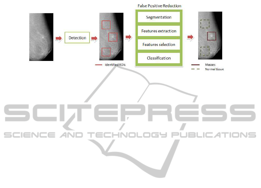
Fig.1. CADe block scheme.

According to BIRADs lexicon [4] there are four different signs of breast disease in

mammograms: masses, architectural distortion, calciﬁcations, focal asymmetry.

– Masses are space occupying lesions seen in two different projections. They can

have: circumscribed margins well-deﬁned or sharply-deﬁned; indistinct margins ill

deﬁned; spiculated margins, when the the lesion is characterized by lines radiating

from the margins of the mass.

– Architectural distortion appear when the normal architecture is distorted with no

deﬁnite mass visible. This includes spiculations radiating from a point, and focal

retraction or distortion at the edge of the parenchyma. Architectural distortion can

also be an associated ﬁnding.

– Focal asymmetry is a density that cannot be accurately described using the other

shapes. It is visible as asymmetry of tissue density with similar shape on two views,

but completely lacking borders and the conspicuity of a true mass. Additional imag-

ing may reveal a true mass or signiﬁcant architectural distortion.

– Calciﬁcations are tiny deposits of calcium in the breast. Malignant calciﬁcations

are classiﬁed into: amorphous or indistinct calciﬁcations often round or “ﬂake”

shaped calciﬁcations; coarse, heterogeneous calciﬁcations, irregular calciﬁcations

with varying sizes and shapes; ﬁne, pleomorphic or branching calciﬁcations, more

conspicuous than the amorphous forms, varying in sizes and shapes. Benign calci-

ﬁcations are usually larger than calciﬁcations associated with malignancy, coarser,

often round with smooth margins and much more easily seen.

In particular, this study is devoted to the automatic massive lesions identiﬁcation by

CADe systems.

2 Methods for the Performance Evaluation

All the images used in this study belong to the Digital Database for Screening Mam-

mography (DDSM) [5]. It contains 2275 studies, with two Cranio-Caudal (CC) views

and two Medio-Lateral Oblique (MLO) views of each breast. The digital database has

been obtained by digitalizing screen ﬁlm mammographic images using four different

scanners devices at three different hospitals in South Florida, with a spatial resolution

in the range [42 − 50] µm and pixel resolution in the range [12 − 16] bpp. Although the

greatest request of the scientiﬁc community is at the moment to consider Direct Dig-

ital Databases, DDSM is the widest public mammographic images database available,

with the most relevant variety of cases, including masses, calciﬁcations and architec-

tural distortions. Each study contains radiologist’s report of the identiﬁed lesions, if

present, including lesion type, position, biopsy proven assessment, boundary, subtlety,

etc., according to BIRADs lexicon third edition. Radiologist’s report can be used as the

ground-truth for the detection procedure, while it would not be enough for the diag-

nosis step, since for example, margins of masses are not drawn accurately. Having the

ground-truth, we can classify each ROI identiﬁed by the algorithm as a True Positive

(TP), a False Positive (FP), or a True Negative (TN) and compute the sensitivity of the

CADe and the number of False Positives per Image (FPpI). This task is recommended

to compare our algorithm to the others proposed in the literature.

3 Mass Identiﬁcation

In the ﬁrst step, a CADe system extracts, from the original mammogram, suspicious

regions on which the radiologists have to focus their attention. The method adopted

for the automatic identiﬁcation of masses in the mammographic images, analyzes the

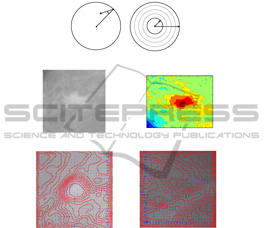
orientation of the gradient vectors in the image using circular support regions, to ﬁnd

highly compact structures with a growing luminance towards their center. The steps of

this procedure are fully described in [6]. Here below, we only recall the basic ideas.

– Decimate the original image. Given the very large size of mammographic images

in DDSM, we reduce resolution to the range [400 − 500] µm. In this way, the

algorithm can still identify the smallest masses with a diameter of 3 mm, but allows

a fast computation.

– Segment the background. We isolate the breast region by implementing an active

contour procedure and histogram thresholding in order to avoid the automatic iden-

tiﬁcation be applied to the ﬁlm background regions.

– Grid the image. Applying the algorithm only on a 5-pixels step grid.

– Consider a circle with radius R around every point (i, j) of the grid and compute

on uniformly distributed N = 24 points on the circle (i.e., every 15 degrees) the

following quantity:

(i, j) =

k,lǫR

cos θ(k, l),

where θ(k, l) is the angle between a gradient vector in (k, l ) and the straight line

connecting the pixels at (i, j) and (k, l) (see Fig. 2 left). The term cos θ(k, l) rep-

resents a measure of the convergence of gradient vectors in the circle to the pixel

of interest (i, j). When x

(i, j) = 1 all the gradient vectors from the circle are

oriented toward the same point. This occurs when the iso-intensity lines are con-

centric. It occurs when the pixel (i, j) is near the center of a massive lesion as one

can see in Fig. 3. Figure 4 shows gradient vectors (blue lines) at every 5 pixels

and iso-intensity lines (red lines) superimposed to a ROI containing a mass and to

a ROI containing only normal tissue.

),( lk

),( ji

gradient

vector

pixel of interest

),( ji

min

max

Fig.2. Deﬁnition of the quantities (left) and iteration for different radii (right).

100 200 300 400 500 600 700

100

200

300

400

500

600

700

Fig.3. A ROI containing a massive lesion (left) and the iso-intensity lines of the same ROI (right).

Fig.4. Two ROIs containing a mass (left) and not a mass (right) with isointensity lines and gra-

dient vectors superimposed.

– Repeat for different radii and compute, for every point (i, j) of the grid, the quan-

tity:

x(i, j) = mean

Rmin<R<Rmax

(i, j).

Because masses have different diameters, from 3 to 40 mm, the region of support

has to be adapted to all the possible sizes of the masses. In particular, we know that

the radius of typical masses is in the range [1.5 − 20] mm that for the considered

not decimated image corresponds to [30 − 400] pixels.

– Sort the results. In a preliminary phase, we show to the radiologist more than one

option. All pixels (i, j) which exceed a certain percentage p of the maximum value

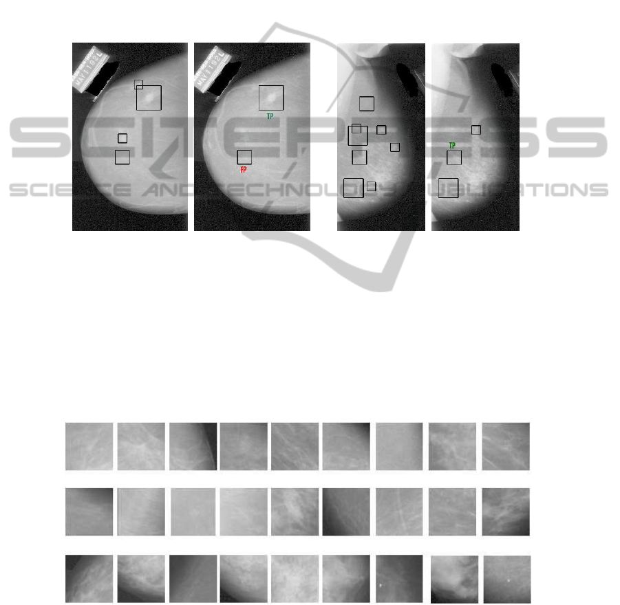
of x(i, j) are presented to the radiologist and labeled in an ascending order: the

more suspicious structures have the bigger markers. So, we have to choose the

parameter p so that x(i, j) > p · ˆx where ˆx is the maximum value of x for every

i, j. Figure 5 shows two examples of the algorithm results: in the ﬁrst case, the

algorithm ﬁnds only one mass that corresponds to the radiologist marker and in the

other case it ﬁnds 3 masses and the correct result is the mass labeled as the ﬁrst. In

our study we use p = 0.80.

– Optimize. All the markers that fall into adjacent centers are grouped to have a more

readable result.

Fig.5. Two examples of the algorithm output.

After the automatic identiﬁcation step, we only consider images where true positives

have been located by the algorithm, in order to separately assess the performance of

the FPR step. So, we consider the better resulting cases, containing 157 ROIs with TPs

and 312 ROIs with FPs. This setting provides an initial sensitivity equal to 1 and a

mean FPpI equal to 2.2. The aim of our study is to reduce the number of FPpI, while

preserving the sensitivity value the highest possible.

In order to introduce the reader to some of the problems encountered with the FPR

step, we report in Fig. 6 some of the ROIs containing a false positive.

Fig.6. Some examples of ROIs containing a false positive sign of disease.

4 Automatic Segmentation

After the identiﬁcation algorithm locates suspicious signs in the mammogram, a ROI

of ﬁxed dimension is extracted around the identiﬁed point. In the following, the ROI

is processed by a Fuzzy C-Means clustering algorithm to implement an intensity-based

segmentation with a number of intensity levels equal to 5. The reconstructed image is

then binarized considering as “foreground” only the largest group of adjacent pixels

belonging to the cluster with the highest luminance level, and as “background” the

remaining ones. Figure 7 shows some examples of the segmentation results for ROIs

containing a mass and ROIs with false positives.

Fig.7. Segmented ROIs containing a mass (left) and not a mass (right).

5 Features Extraction

The approach used in this work consists in testing a large set of features and then apply-

ing an automatic features selection algorithm in order to deﬁne a proper set of features

with respect to a given training set. After the segmentation of the mass boundary, we

have extracted the following features:

– Morphological features including area, circularity, eccentricity, roughness of the

contour, elongation;

– Law’s texture features [7]. Law proposed a method for classifying each pixel in

an image based upon measures of local texture energy. The texture energy features

represent the amounts of variation within a sliding window applied to several ﬁl-

tered versions of the given image. These measures are computed by ﬁrst applying

small convolution kernels to the image, and then performing a nonlinear window-

ing operation. The 2-D convolution kernels typically used for texture discrimina-

tion are generated from the following set of one-dimensional convolution kernels of

length 5: L5 = [1, 4, 6, 4, 1], E5 = [−1, −2, 0, 2, 1], S5 = [−1, 0, 2, 0, −1],

R5 = [1, −4, 6, −4, 1], W 5 = [−1, 2, 0, − 2, 1]. The operators listed above per-

form the detection of the following types of features: L5 local average (or level),

E5 edges, S5 spots, R5 ripples, W 5 waves. By combining in a nonlinear manner

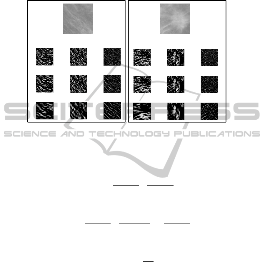
the above ﬁlters, we obtain 14 Texture Energy Measures (TEM) images. The most

representatives are reported in Fig. 8 for a ROI containing an oriented pattern and

one with a mass. Finally, for each of the 14 images, the following parameters are

evaluated: mean, variance, kurtosis, and skewness.

E5L5 S5L5 W5L5 R5L5

E5W5E5R5 S5W5 S5R5 W5R5

E5L5 S5L5 W5L5 R5L5 E5S5

E5W5 E5R5 S5W5 S5R5 W5R5

E5S5

Fig.8. Laws’ texture energy measure for a ROI with a mass (bottom) and one with an oriented

patter (up).

– Haralick texture features [8] are computed on the co-occurrence matrix extracted

from the original ROI, from the ROI transformed by nonlinear contrast enhance-

ment, from the ROIs transformedby the Ranklet Transform [9], and ﬁnally from the

ROI elaborated by Sobel ﬁlters at different sizes. In particular, the ranklet transform

is an orientation-selective, non-parametric and multi-resolution transform which

has already been successfully exploited in image classiﬁcation tasks, speciﬁcally

face recognition in image frames [10]. The ranklet transform of an image involves

three phases: multiresolution, orientation-selective, and non-parametric analysis.

Fig. 9 shows some examples of the same ROIs above processed by Ranklet trans-

form, at three different resolution factors (4, 6, and 14).

6 Features Selection

At a preliminary step, more than 1000 features have been extracted and a ranking by

a speciﬁc selection criterion has been applied on this set. Features have been evalu-

ated one by one, in order to assign a score to each of them according to its relevance,

evaluated on a training set.

Three indexes have been computed in this study, leading to different working points

(i.e., different possible trades off among the ability of reducing false positives, while

preserving true positives):

Horizontal RES 4 Vertical RES 4 Diagonal RES 4

Horizontal RES 6 Vertical RES 6 Diagonal RES 6

Horizontal RES 14 Vertical RES 14 Diagonal RES 14

Horizontal RES 4 Vertical RES 4 Diagonal RES 4

Horizontal RES 6 Vertical RES 6 Diagonal RES 6

Horizontal RES 14 Vertical RES 14 Diagonal RES 14

Fig.9. Ranklet transform at three different resolutions of a ROI with a mass (bottom) and one

with an oriented pattern (up).

– the difference between the rate of ROIs correctly recognized as normal tissue in the

initial amount of false positives and the rate of wrongly recognized ROIs as normal

tissue in the initial amount of true positives:

IN D

T N

T N + F P

−

F N

T P + F N

;

– the difference between the improvement of the correctness and the decrease of the

sensitivity:

IN D



T P

T P + F P

−

sT P

sT P + sF P





T P

T P + F N

− 1



;

– how much the false positive reduction is stronger than the loss of false positives,

leading to an increasing of false negative ROIs:

IN D

= 1 −

F N

T N

;

Using the cited indexes,we denote the three differentranking vectors as RKC

, RKC

and RKC

As last step, it was necessary to ﬁnd out the optimal number of features among

those ranked. Actually, the performance of the system can not be uniquely assessed,

because they depend on the radiologist’s needs and expectation. The radiologist, in fact,

could require the CADe system providing the minimum number of False Positives per

mammogram, that is the maximum reduction of the number of FPpI even in spite of a

reduction of sensitivity, in order to avoid too much false suggestions which could divert

away attention from the real mass. Otherwise, the radiologist may not require ﬁrst of

all any losses of sensitivity, even at the expense of a low reduction of false positives. In

this case, the radiologist prefers receiving even many suggestions but always including

the real mass, when it is present. Section 8 will provide some numerical examples for

these options.

7 Fuzzy Classiﬁcation

A Fuzzy Inference System (FIS) has been implemented and used for the classiﬁcation

of ROIs into abnormal or normal breast tissue [11]. To decide an appropriate diagnosis

in one patient, we introduce three non-fuzzy sets, as explained in [11].

– The set of symptoms (corresponding to the set of features) S = {S

, S

, ..., S

– The set of diagnosis D = {D

, D

, ..., D

} (where, in this case, p = 2 because of

the presence of two classes, “Cancer (C)” or “Normal (N)” that is ROI containing

a mass or ROI containing normal tissue).

– The set of patients P = {P

} (the set of ROIs cropped from the mammograms of

a patient).

The assignment of a diagnosis to the patient requires the evaluation of two distinct rela-

tions: the Patient-Symptom Relation (P S) where the different symptoms are evaluated

in the mammograms of the considered patient; the Symptom-Diagnosis Relation (SD)

where the importance of each symptom for the diagnosis (C or N) is evaluated. This

procedure is at a preliminary investigation stage, and at present it computes simply the

positive predictive value and the negative predictive values of each feature indepen-

dently, for each patient in the training set, leading to the so called incidence level of the

symptom to the diagnosis. Hence, the symptoms occurring in a set S are associated with

the diagnosis from set D (SD ) and further they are associated in turn with the patient P

(assuming that information about all symptoms in S is complete in the patient’s case),

in order to establish the ﬁnal Patient-Diagnosis Relation (P D).

7.1 Fuzzy Inference Engine

A necessary step for the implementation of a FIS is the deﬁnition of a set of fuzzy

rules which relate the input values (the symptoms) to the output values (the diagnoses).

The fuzzy rules are deﬁned according to the two above described relations and clinical

experience, according to [11]. In particular the following rules

if (symptom S

is a decisive feature for diagnosis B)

| {z }

SD relation

and (symptom S

is present in patient P )

| {z }

P S relation

then (diagnosis B is assign ed to patient P )

| {z }

P D relation

are deﬁned, which consider only one symptom at a time. In general, for each symptom,

4 rules could be written which combine N and M diagnoses and low and high presence

of the symptom in the patient. However, the experience and the data lead to conclude

that, for a certain symptom S

, low means presence of mass and high means normal

tissue, or vice versa. Hence, only a subset of possible rules are implemented. In the

considered application, the output values are crisp (either N or M). This means that

the considered FIS is simpliﬁed with respect to the general case where also the output

variables are fuzzy sets. Hence, the defuzziﬁcation step is not required and, in order to

associate the ﬁnal membership degrees to the two ﬁnal diagnoses (N , M), the following

quantities can be considered [11]:

opt

j=1

IL(S

) · µ

l/h

)

opt

j=1

IL(S

)

opt

j=1

IL(S

) · µ

l/h

)

opt

j=1

IL(S

)

where N

opt

is the selected optimal number of features ranked according to one of the

three criterions shown above, and IL(S

N/M

) denotes the incidence of feature S

the diagnosis N/M. µ

provides the degree of not abnormality of the considered ROI,

while µ

provides the degree of abnormality of the same ROI. So, the outputs of the

fuzzy inference system are: the credibility degree that the ROI is a mass (µ

) and

the credibility degree that the same ROI is normal breast tissue (µ

). Differently from

standard classiﬁers, these two indexes are not complementary to the unity. These values

have to be compared to provide the ﬁnal decision.

8 Results

For the performance evaluation of the fuzzy classiﬁer, a leave-one-out cross-validation

technique has been adopted: the training set was composed of the entire dataset of ROIs

except one which is used as test. This procedure is repeated for each features vector

in the training set. The optimal number of features to be used is different according

to the ranking and to the selection criterion. In particular, using the same criterion for

both ranking and selection of the optimal number, we obtain NP

opt

= 90 for crite-

rion IND

, NP

opt

= 39 for criterion IND

, and NP

opt

= 27 for criterion IND

The results of the classiﬁcation using the three methods are reported in Table 1, in the

columns identiﬁed with No Threshold. It means that the ﬁnal decision is taken only by

comparing credibility degrees of abnormality and of not abnormality.

8.1 Uncertain Diagnosis: Certainty Threshold

The reported results exhibit a sensitivity always greater than 0.8 and a correctness

increased from 0.33 up to 0.5-0.7, with a number of FPpI that varies according to the

used criterion in the range [0.3 − 0.97]. Moreover, another important aspect has to be

considered. The fuzzy logic classiﬁer assigns to each ROI under analysis two values

thus not conferring a single judgment of membership to a class. These membership

degrees have to be compared to make a decision, but this comparison can not be suf-

ﬁcient. It is important to analyze the difference between µ

and µ

in order to take

into account the natural variability of these degrees. Hence a certainty threshold has

been empirically set to 0.15. This threshold has been set low enough in order to exclude

just the most evident doubtful cases. If the absolute value of (µ

− µ

) was less than

0.15, a conservative choice is to classify the ROI as abnormal. Thus, every doubtful

case can be further analyzed by the radiologist or by the computerized system. Table 1

shows the results obtained adopting this modiﬁed approach, in the columns identiﬁed

by Threshold. Using this threshold, the number of positives increases, thus causing the

Table 1. Results of classiﬁcation with a certainty threshold equal to 0.15, compared with the

previous results without any threshold.

I N D

Threshold No Threshold Threshold No Threshold Threshold No Threshold

TP 147 126 157 153 157 156

FN 10 31 0 4 0 1

TN 210 264 183 198 105 159

FP 102 48 129 114 207 153

SENS 0.9363 0.8025 1 0.9745 1 0.9936

FPpI 0.65 0.30 0.82 0.72 1.31 0.97

increase in both True Positives and False Positives with respect to the No Threshold

case. At the same time, the working point shifts toward a greater sensitivity, with an

acceptable increase in F P pI. All these results prove that the features ranking/selection

algorithms, the fuzzy classiﬁer, and the conservative setting achieved by the certainty

threshold perform well and can be easily adapted to different requirements of the radi-

ologists assigning to the CADe a good ﬂexibility and adaptability to different clinical

scenarios.

9 Comparisons

We report also the most relevant results described in the literature concerning the False

Positive Reduction in the automatic detection of breast masses. In particular, Li et

al. [12] used a soft neural network decision classiﬁcation. Angelini et al. [13] proposed

a support vector regression ﬁltering approach. Masotti et al. [9] reduced false positives

via gray scale invariant ranklet texture features using a support vector machine clas-

siﬁer for discrimination. Tourassi et al. [14] used a template matching scheme based

on mutual information. Varela et al. [15] employed a neural network classiﬁer to merge

different combination of features. All the results are compared in Table 2 in terms of the

True Positive Reduction (TPR) and the False Positive Reduction (FPR). The number of

ROIs used in the studies is also reported. We also insert our results obtained by criterion

IN D

10 Conclusions

In this work, we presented a study on the False Positives Reduction in the automatic

breast masses identiﬁcation in mammographic images. We addressed the FPR step as

Table 2. Comparisons of different methods for false positive reduction.

TPR FPR ROIs

Li et al. 1% 56% 25

Angelini et al. 13% 38% 69

Tourassi et al. 10% 65% 1820

Varela et al. 22% 85% 120

Masotti et al. 0% 30% 884

Proposed method 0% 58% 469

a two classes classiﬁcation problem, with the aim to assign to each suspicious ROI a

degree of abnormality and a degree of not abnormality, thus reducing the whole number

of ROIs to be presented to the radiologist. A large set of features have been extracted

from the ROIs identiﬁed by an automatic identiﬁcation algorithm proposed by the au-

thors. Then, the selected features have been used to train a fuzzy classiﬁer, properly

structured for medical applications. Different working points have been considered so

that the radiologist could choose the best tradeoff between sensitivity and false positive

per image, according to the clinical application.

References

1. M. Bazzocchi and F. Mazzarella, “CAD systems for mammography: a real opportunity? A

review of the literature,” http://www.springerlink.com/content/x3157r8u72196h45/

fulltext.pdf/, 2006.

2. A. Oliver, “A new approach to the classiﬁcation of mammographic masses and normal breast

tissue,” in Proceedings of the 18th International Conference on Pattern Recognition, 2006,

vol. 4, pp. 707 – 710.

3. J. Wei, H-P. Chan, B. Sahiner, C. Zhou, and L. M. Hadjiiski, “Computer-aided detection

of breast masses on mammograms: Dual system approach with two-view analysis,” Med.

Phys., vol. 36, no. 10, pp. 4451 – 4460, 2009.

4. C. Balleyguier, S. Ayadi, K. Van Nguyen, D. Vanel, C. Dromain, and R. Sigal, “BIRADS

classiﬁcation in mammography,” European Journal of Radiology, vol. 61, pp. 192–194,

2007.

5. University of South Florida, “DDSM: Digital database for screening mammography,”

http://marathon.csee.usf.edu/Mammography/Database.html, 2000.

6. A. Mencattini, G. Rabottino, M. Salmeri, and R. Lojacono, “Assessment of a breast masses

identiﬁcation procedure using an iris detector,” IEEE Transactions on Instrumentation and

Measurement, in press.

7. K. I. Laws, “Laws’ texture measures,” http://www.ccs3.lanl.gov/ kelly/ZTRANSITION/

notebook/laws.shtml, 2001.

8. R. M. Haralick, “Statistical and structural approaches to texture,” Proceedings of the IEEE,

vol. 67, no. 5, pp. 786 – 804, 1979.

9. M. Masotti, N. Lanconelli, and R. Campanini, “Computer aided mass detection in mammog-

raphy: False positive reduction via gray scale invariant ranklet texture features,” Medical

Physics, vol. 36, no. 2, 2009.

10. F. Smeraldi, “Ranklets: Orientation selective non-parametric features applied to face de-

tection,” in 16th International Conference on Pattern Recognition, 2002, vol. 3, pp. 351 –

359.

11. E. Rakus-Andersson, Fuzzy and rough techniques in Medical Diagnosis and Medication,

Springer-Verlag, 2007.

12. L. Li, Y. Zheng, L. Zhang, and R. A. Clark, “False-positive reduction in cad mass detection

using a competitive classiﬁcation strategy,” Medical Physics, vol. 28, 2001.

13. E. Angelini, R. Campanini, and A. Riccardi, “Support vector regression ﬁltering

for reduction of false positives in a mass detection cad scheme: Preliminary results,”

http://amsacta.cib.unibo.it/archive/00000912/01/angelini05support.pdf, 2005.

14. G. D. Tourassi, R. Vargas-Vorecek, D. M. Catarious, and C. E. Floyd, “Computer assisted

detection of mammographic masses: a template matching scheme based on mutual informa-

tion,” Medical Physics, vol. 30, no. 8, pp. 2123 – 2130, 2003.

15. C. Varela, P. G. Tahoces, A. J. Mendez, M. Souto, and J. J. Vidal, “Computerized detection

of breast masses in mammograms,” Computers in Biology and Medicine, vol. 37, pp. 214 –

226, 2007.