
SPEEDING UP LATENT SEMANTIC ANALYSIS
A Streamed Distributed Algorithm for SVD Updates
Radim
ˇ
Reh˚uˇrek
NLP lab, Masaryk University in Brno, Brno, Czech Republic
Keywords:
Distributed LSA, Streamed SVD, One-pass SVD, Matrix decomposition, Subspace tracking.
Abstract:
Since its inception 20 years ago, Latent Semantic Analysis (LSA) has become a standard tool for robust,
unsupervised inference of semantic structure from text corpora. At the core of LSA is the Singular Value
Decomposition algorithm (SVD), a linear algebra routine for matrix factorization. This paper introduces a
streamed distributed algorithm for incremental updates, which allows the factorization to be computed rapidly
in a single pass over the input matrix on a cluster of autonomous computers.
1 INTRODUCTION
The purpose of Latent Semantic Analysis (LSA) is to
find hidden (latent) structure in a collection of texts
represented in the Vector Space Model (Salton, 1989).
LSA was introduced in (Deerwester et al., 1990) and
has since become a standard tool in the field of Nat-
ural Language Processing and Information Retrieval.
At the heart of LSA lies the Singular Value Decom-
position algorithm, which makes LSA (sometimes
also called Latent Semantic Indexing, or LSI) really
just another member of the broad family of applica-
tions that make use of SVD’s robust and mathemat-
ically well-founded approximation capabilities
1
. In
this way, although we will discuss our results in the
perspectiveand terminology of LSA and Natural Lan-
guage Processing, our results are in fact applicable to
a wide range of problems and domains across much
of the field of Computer Science.
1.1 Singular Value Decomposition
Latent Semantic Analysis assumes that each docu-
ment (observation) can be described using a fixed set
of real-valued features (variables). These features
capture the usage frequency of distinct words in the
document, and are typically re-scaled by some TF-
IDF scheme (Salton, 1989). However, no assumption
1
Another member of that family is the discrete KarhunenLove
Transform, from Image Processing; or Signal Processing, where
SVD is commonly used to separate signal from noise. SVD is
also used in solving shift-invariant differential equations, in Geo-
physics, in Antenna Array Processing, ...
is made on what the particular features are or how
to extract them from raw data—LSA simply repre-
sents the input data collection of n documents, each
described by m features, as a matrix A ∈ R
m×n
, with
documents as columns and features as rows.
In theory, the term-document matrix A can be di-
rectly mapped to physical memory and processed.
However, A is commonly left implicit, as it is often
distributed among many computers, unknown in its
entirety and/or computed partially on-demand. In-
deed, in many cases the implied matrix is even infinite
in size, gradually growing as the collection grows.
Nevertheless, there is a reason why it is worth-
while to view the collection as a single gigantic ma-
trix. It allows us to consider linear algebra decompo-
sition algorithms that provide succint, mathematically
well-founded ways of discovering latent structure of
the matrix and, thereby, of the original data collection.
In case of LSA, the algorithm of choice is the Singu-
lar Value Decomposition, SVD. Assuming n ≫ m, the
SVD of A yields A
m×n
= U
m×m
S
m×m
V
T
m×n
, where U,
V are orthogonal matrices (called left and right sin-
gular vectors) and S is a diagonal matrix of singular
values with diagonal entries in decreasing order.
Here and elsewhere, we use the subscripts A
x×y
to
denote that matrix A has x rows and y columns but
omit the subscripts whenever there is no risk of con-
fusion.
1.2 Related Work
Historically, most research on SVD optimization has
gone into Krylov subspace methods, such as Lanczos-
446
ˇ
Reh˚u
ˇ
rek R..
SPEEDING UP LATENT SEMANTIC ANALYSIS - A Streamed Distributed Algorithm for SVD Updates.
DOI: 10.5220/0003191304460451
In Proceedings of the 3rd International Conference on Agents and Artificial Intelligence (ICAART-2011), pages 446-451
ISBN: 978-989-8425-40-9
Copyright
c
2011 SCITEPRESS (Science and Technology Publications, Lda.)

based iterative solvers (see e.g. (Vigna, 2008) for
a recent large-scale SVD effort). Our problem is,
however, different in that we can only afford a sin-
gle pass over the input corpus (iterative solvers re-
quire O(k) passes in general). Our scenario, where
the decomposition must be updated on-the-fly and
in constant memory, as the stream of observations
cannot be repeated or even stored in off-core mem-
ory, can be viewed as an instance of subspace track-
ing. See (Comon and Golub, 1990) for an excellent
overview on the complexity of various forms of ma-
trix decomposition algorithms in the context of sub-
space tracking.
An explicitly formulated O(m(k + c)
2
) method
(where c is the number of newly added documents)
for incremental LSA updates is presented in (Zha and
Simon, 1999). They also give formulas for updating
rows of A as well as rescaling row weights. Their al-
gorithm is completely streamed and runs in constant
memory. It can therefore also be used for online sub-
space tracking, by simply ignoring all updates to the
right singular vectors V. The complexity of updates
was further reduced in (Brand, 2006) who proposed
a linear O(mkc) update algorithm by a series of c fast
rank-1 updates. However, in the process, the ability to
track subspaces is lost (despite their tentative claim to
the contrary). Their approach is akin to the k-Nearest
Neighbours (k-NN) method of Machine Learning: the
lightning speed during training is offset by memory
requirements of storing the intermediate model.
These incremental methods concern themselves
with adding new documents to an existing decompo-
sition. What is needed for a distributed version of
LSA is a slightly different task: given two existing
decompositions, merge them together into one. We
did not find any explicit, efficient algorithm for merg-
ing decompositions in the literature. In this research
paper we therefore seek to close this gap, provide
such algorithm and use it for computing distributed
LSA. The following section describes the algorithm
and states conditions under which the merging makes
sense when dealing with only truncated rank-k ap-
proximation of the decomposition.
2 DISTRIBUTED LSA
In this section, we derive an algorithm for distributed
computing of LSA over a cluster of autonomous com-
puters.
2.1 Algorithm Overview
Parallel computation will be achieved by column-
partitioning the input matrix A into several
smaller submatrices, called jobs, A
m×n
=
h
A
m×c
1
1
,A
m×c
2
2
,··· ,A
m×c
j
j
i
,
∑
c
i
= n. Since columns
of A correspond to documents, each job A
i
amounts to
processing a chunk of c
i
input documents. The sizes
of these chunks are chosen to fit available resources
of the processing nodes: bigger chunks mean faster
overall processing but on the other hand consume
more memory.
Jobs are then distributed among the available clus-
ter nodes, in no particular order, so that each node will
be processing a different set of column-blocksfrom A.
The nodes need not process the same number of jobs,
nor process jobs at the same speed; the computations
are completely asynchronous and independent. Once
all jobs have been processed, the decompositions ac-
cumulated in each node will be merged into a single,
final decomposition P = (U,S).
What is needed are thus two algorithms:
1. Find P
i
= (U
m×c
i
i
,S
c
i
×c
i
i
) eigen decomposition of
a single job A
m×c
i
i
such that A
i
A
T
i
= U
i
S
2
i
U
T
i
.
These P
i
decompositions will form the base case
for merging.
2. Merge two decompositions P
i
= (U
i
,S
i
), P
j
=
(U
j
,S
j
) of two jobs A
i
, A
j
into a single decom-
position P = (U, S) such that
A
i
,A
j
A
i
,A
j
T
=
US
2
U
T
.
We’d like to highlight the fact that the first algo-
rithm will perform decomposition of a sparse input
matrix; the second algorithm will merge two dense
decompositions into another dense decomposition.
This is in contrast to incremental updates discussed
in the literature (Levy and Lindenbaum, 2000; Zha
and Simon, 1999; Brand, 2006), where the existing
decomposition and the new documents are mashed to-
gether into a single matrix, losing any potential bene-
fits of sparsity.
2.2 Solving the Base Case
In LSA (using the same notation introduced in Sec-
tion 1), the truncation factor k is typically in the hun-
dreds or thousands, the number of features m be-
tween 10
4
to 10
6
and the number of documents n
tends to infinity, so that k ≪ m ≪ n. Density of the
job matrices is well below 1%, so a sparse solver is
called for, that makes efficient use of the sparse ma-
trix structure. Also, a direct sparse SVD solver of A
i
is preferable to the roundabout eigen decomposition
of A
i
A
T
i
, for memory-conserving as well as numeri-
cal accuracy reasons (see e.g. (Golub and Van Loan,
1996)). Finally, because k ≪ m, a partial decompo-
sition is required which only returns the k greatest
SPEEDING UP LATENT SEMANTIC ANALYSIS - A Streamed Distributed Algorithm for SVD Updates
447

factors—computing the full spectrum would be a ter-
rible overkill.
For these reasons, we solve base cases with a
“black-box” in-core sparse partial SVD algorithm.
2.3 Merging Decompositions
No explicit algorithm (as far as we know) exists for
merging two truncated eigen decompositions(or SVD
decompositions) into one. We therefore propose our
own, novel algorithm here, starting with its derivation
and summing up the final version in the end.
The problem can be stated as follows. Given two
truncated eigen decompositions P
1
= (U
m×k
1
1
,S
k
1
×k
1
1
),
P
2
= (U
m×k
2
2
,S
k
2
×k
2
2
), which come from the (by now
lost and unavailable) input matrices A
m×c
1
1
, A
m×c
2
2
,
k
1
≤ c
1
and k
2
≤ c
2
, find P = (U,S) that is the eigen
decomposition of
A
1
,A
2
.
Our first approximation will be the direct naive
U,S
2
eigen
←−−−
U
1
S
1
,U
2
S
2
U
1
S
1
,U
2
S
2
T
. (1)
This is terribly inefficient, and forming the ma-
trix product of size m × m on the right hand side is
prohibitively expensive. Writing SVD
k
for truncated
SVD that returns only the k greatest singular numbers
and their associated singular vectors, we can equiva-
lently write:
Algorithm 1: SVD merge.
Input: Truncation factor k, Decay factor γ,
P
1
= (U
m×k
1
1
,S
k
1
×k
1
1
), P
2
= (U
m×k
2
2
,S
k
2
×k
2
2
)
Output: P = (U
m×k
,S
k×k
)
U,S,V
T
SVD
k
←−−−
γU
1
S
1
,U
2
S
2
1
This is more reasonable, with the added bonus of
increased numerical accuracy over the related eigen
decomposition. Note, however, that the computed
right singular vectors V
T
are not used at all, which
is a sign of further inefficiency. This leads us to break
the algorithm into several steps:
Algorithm 2: QR merge.
Input: Truncation factor k, Decay factor γ,
P
1
= (U
m×k
1
1
,S
k
1
×k
1
1
), P
2
= (U
m×k
2
2
,S
k
2
×k
2
2
)
Output: P = (U
m×k
,S
k×k
)
Q,R
QR
←−−
γU
1
S
1
,U
2
S
2
1
U
R
,S,V
T
R
SVD
k
←−−− R2
U
m×k
← Q
m×(k
1
+k
2
)
U
(k
1
+k
2
)×k
R
3
On line 1, an orthonormal subspace basis Q is
found which spans both of the subspaces defined by
columns of U
1
and U
2
, span(Q) = span(
U
1
,U
2
).
Multiplications by S
1
, S
2
and γ provide scaling for R
only and do not affect Q in any way, as Q will always
be orthogonal (with columns of unit length). Our al-
gorithm of choice for constructing the new basis is
QR factorization, because we can use its other prod-
uct, the upper trapezoidal matrix R, to our advantage.
Now we’re almost ready to declare (Q,R) our target
decomposition (U,S), except R is not diagonal. To
diagonalize R, we perform an SVD on it, on line 2.
This gives us the singular values S we need as well
as the rotation of Q necessary to represent the ba-
sis in this new subspace. The rotation is applied on
line 3. Finally, both output matrices are truncated to
the requested rank k. The costs are O(m(k
1
+ k
2
)
2
),
O((k
1
+ k
2
)
3
) and O(m(k
1
+ k
2
)
2
) for line 1, 2 and 3
respectively, for a combined total of O(m(k
1
+ k
2
)
2
).
Although more elegant than Algorithm 1, the
baseline algorithm is only marginally more efficient
than a direct SVD. This comes as no surprise, as the
two algorithms are quite similar and SVD of rectangu-
lar matrices is often internally implemented by means
of QR in exactly this way. Luckily, we can do better.
First, we observe that the QR decomposition
makes no use of the fact that U
1
and U
2
are already
orthogonal. Capitalizing on this will allow us to
represent U as an update to the existing basis U
1
,
U =
U
1
,U
′
, dropping the complexity of the first
step to O(mk
2
2
). Secondly, the application of rota-
tionU
R
toU can be rewritten as UU
R
=
U
1
,U
′
U
R
=
U
1
R
1
+U
′
R
2
, dropping the complexity of the last step
to O(mkk
1
+ mkk
2
). Plus, the algorithm can be made
to work by modifying the existing matrices U
1
,U
2
in
place inside BLAS routines, which is a considerable
practical improvement over Algorithm 2, which re-
quires allocating additional m(k
1
+ k
2
) floats.
Algorithm 3: Optimized merge.
Input: Truncation factor k, Decay factor γ,
P
1
= (U
m×k
1
1
,S
k
1
×k
1
1
), P
2
= (U
m×k
2
2
,S
k
2
×k
2
2
)
Output: P = (U
m×k
,S
k×k
)
Z
k
1
×k
2
← U
T
1
U
2
1
U
′
,R
QR
←−− U
2
−U
1
Z2
U
R
,S,V
T
R
SVD
k
←−−−
γS
1
ZS
2
0 RS
2
(k
1
+k
2
)×(k
1
+k
2
)
3
"
R
k
1
×k
1
R
k
2
×k
2
#
= U
R
4
U ← U
1
R
1
+U
′
R
2
5
The first two lines construct orthonormal basis U
′
for the component of U
2
that is orthogonal to U
1
,
ICAART 2011 - 3rd International Conference on Agents and Artificial Intelligence
448

span(U
′
) = span((I −U
1
U
T
1
)U
2
) (2)
= span(U
2
−U
1
(U
T
1
U
2
)). (3)
As before, we use QR factorization because the
upper trapezoidal matrix R will come in handy when
determining the singular vectors S.
Line 3 is perhaps the least obvious, but follows
from the requirement that the updated basis
U,U
′
must satisfy
U
1
S
1
,U
2
S
2
=
U
1
,U
′
X, (4)
so that
X =
U
1
,U
′
T
U
1
S
1
,U
2
S
2
. (5)
By multiplying,
U
T
1
U
′T
U
1
S
1
,U
2
S
2
=
U
T
1
U
1
S
1
U
T
1
U
2
S
2
U
′T
U
1
U
′T
U
2
S
2
(6)
and using the equalities R = U
′T
U
2
, U
′T
U
1
= 0
and U
T
1
U
1
= I (all by construction) we obtain
X =
S
1
U
T
1
U
2
S
2
0 U
′T
U
2
S
2
=
S
1
ZS
2
0 RS
2
. (7)
Line 4 is just a way of saying that on line 5, U
1
will be multiplied by the first k
1
rows of U
R
, while U
′
will be multiplied by the remaining k
2
rows.
Finally, line 5 seeks to avoid realizing the full
U
1
,U
′
matrix in memory and is a direct application
of the equality
U
1
,U
′
m×(k
1
+k
2
)
U
(k
1
+k
2
)×k
R
= U
1
R
1
+U
′
R
2
. (8)
As for complexity of this algorithm, it is again
dominated by the matrix products and the dense
QR factorization, but this time only of a matrix of
size m × k
2
. The SVD of line 3 is a negligible
O(k
1
+ k
2
)
3
, and the final basis rotation comes up to
O(mk max(k
1
,k
2
)). Overall, with k
1
≈ k
2
≈ k, this is
an O(mk
2
) algorithm.
2.4 Effects of Truncation
While the equations above are provably correct when
using matrices of full rank (putting aside the techni-
cal question of gradual loss of accuracy due to finite
machine precision and rounding errors for now), it is
not at all clear how to justify truncating all interme-
diate matrices to rank k in each update. What effect
does this have on the merged decomposition? How do
these effects stack up as we perform several updates
in succession?
In (Zha and Zhang, 2000), the authors did the hard
work and identified conditions under which operating
with truncated matrices produces exact results. More-
over, they show by way of perturbation analysis that
the results are stable (though no longer exact) even
if the input matrix only approximately satisfies this
condition. They investigate matrices of the so-called
low-rank-plus-shift structure, which (approximately)
satisfy
A
T
A/m ≈ CWC
T
+ σ
2
I
n
, (9)
where C, W are of rank k, W positive semi-
definite, σ
2
the variance of noise. That is, A
T
A can
be expressed as a sum of a low-rank matrix and a
multiple of the identity matrix. They show that ma-
trices coming from natural language corpora do in-
deed possess this structure and that in this case, a
rank-k approximation of A can be expressed as a com-
bination of rank-k approximations of its submatrices
A =
A
1
,A
2
without a serious loss of precision.
2.5 Putting It Together
Let N = {N
1
,...,N
p
} be the p available cluster nodes.
Each node will be processing incoming jobs sequen-
tially, running the base case decomposition from Sec-
tion 2.2 followed by merging the result with the cur-
rent decomposition by means of Algorithm 1, 2 or 3:
Algorithm 4: LSA Node.
Input: Truncation factor k, Queue of jobs A
1
,A
2
,...
Output: P = (U
m×k
,S
k×k
) decomposition of
A
1
,A
2
,...
P = (U,S) ← 0
m×k
,0
k×k
1
foreach job A
i
do2
P
′
= (U
′
,S
′
) ← BaseCase Decomposition(k,A
i
)3
P ← Merge Algo{1,2,3}(k, P,P
′
)4
end5
To construct decomposition of the full matrix A,
we let the nodes work in parallel, distributing the jobs
as soon as they arrive, to whichever node seems idle.
We do not describe the technical issues of load bal-
ancing and recovery from node failure here, but stan-
dard practices apply. Once we have processed all the
jobs (or temporarily exhausted the input job queue, in
the infinite streaming scenario), we merge their indi-
vidual results into one:
Algorithm 5: Distributed LSA.
Input: Truncation factor k, Queue of jobs
A =
A
1
,A
2
,...
Output: P = (U
m×k
,S
k×k
) decomposition of A
P
i
= (U
i
,S
i
) ← LSA Node Algo4(k, subset of jobs1
from A), for i = 1,... , p
P ← Reduce(Merge Algo,
P
1
,... , P
p
)
2
SPEEDING UP LATENT SEMANTIC ANALYSIS - A Streamed Distributed Algorithm for SVD Updates
449

Here, line 1 is executed in parallel, making use of
all p nodes at once, and is the source of parallelism of
the algorithm. On line two, Reduce applies the func-
tion that is its first argument cummulatively to the se-
quence that is its second argument, so that it effec-
tively merges P
1
with P
2
, followed by merging that
result with P
3
, etc.
We note that other divide-and-conquer schemes
are also possible, such as one where the merging in
line 2 of Algorithm 5 happens on pairs of decompo-
sitions coming from approximately the same number
of input documents, so that the two sets of singular
values are of comparable magnitude. Doing so could
lead to improved numerical properties, but we have
not investigated this effect yet.
The algorithm is formulated in terms of a (poten-
tially infinite) sequence of jobs, so that when more
jobs arrive, we can continue updating the decomposi-
tion in a natural way. The whole algorithm can in fact
act as a continuousdaemon service, providing decom-
position of all the jobs processed so far on demand.
3 EXPERIMENTS
In this section, we describe a set of experiments mea-
suring numerical accuracy of the proposed algorithm.
In all experiments, the decay factor γ is set to 1.0,
that is, there is no discounting in favour of new obser-
vation. The number of requested factors is k = 200 in
all cases.
3.1 Set Up
We will be comparing four implementations for par-
tial Singular Value Decomposition:
SVDLIBC A direct sparse SVD implementation due
to Douglas Rohde
2
. SVDLIBC is based on the
SVDPACK package by Michael Berry (Berry,
1992). We use the LAS2 routine (Lanczos of the
related implicit A
T
A or AA
T
matrix with selective
orthogonalizations) to retrieve only the k domi-
nant singular triplets. The implementation works
in-core and therefore doesn’t scale.
ZMS Implementationof the incremental one-pass al-
gorithm from (Zha et al., 1998). The right singular
vectors and their updates are completely ignored
so that our implementation of their algorithm also
realizes subspace tracking.
DLSA Our proposed method. We will be evalu-
ating three different versions of merging, Algo-
rithms 1, 2 and 3, calling them DLSA
1
, DLSA
2
and
2
http://tedlab.mit.edu/∼dr/SVDLIBC/
DLSA
3
in the results, respectively. Sparse SVD
during base case decomposition is realized by an
adapted LAS2 routine from SVDLIBC, see above.
With the exception of SVDLIBC, all the other al-
gorithms operate in a streaming fashion (ehek and So-
jka, 2010), so that the corpus need not reside in core
memory all at once. Although memory footprint of
all algorithms is independent of the size of the cor-
pus, it is still linear in the number of features, O(m).
It is assumed that the decomposition (U
m×k
,S
k×k
) fits
entirely into core memory.
For the experiments, we will be using a corpus of
3,494 mathematical articles collected from the digi-
tal libraries of NUMDAM, arXiv and DML-CZ. Af-
ter the standard procedure of pruning out word types
that are too infrequent (hapax legomena, typos, OCR
errors, etc.) or too frequent (stop words), we are
left with 39,022 distinct features. The final matrix
A
39,022×3,494
has 1.5 million non-zero entries. This
corpus was chosen so that it fits into core memory of
a single computer and its decomposition can there-
fore be computed directly. This will allow us to es-
tablish the “ground-truth” decomposition and set an
upper bound on achievable accuracy and speed.
3.2 Accuracy
Figure 1 plots the relative accuracy of singular val-
ues found by DLSA, ZMS, SVDLIBC and HEBB al-
gorithms compared to known, “ground-truth” values
S
G
. We measure accuracy of the computed singular
values S as r i = |s i − s G i|/s G i, for i = 1, ..., k.
The ground-truth singular values S
G
are computed di-
rectly with LAPACK’s DGESVD routine.
We observe that the largest singular values are
practically always exact, and accuracy quickly de-
grades towards the end of the returned spectrum. This
leads us to the following refinement: When request-
ing x factors, compute the truncated updates for k > x,
such as k = 2x, and discard the extra x− k factors only
when the final projection is actually needed. The er-
ror is then below 5%, which is comparable to the ZMS
algorithm (while DLSA is at least an order of magni-
tude faster even without any parallelization).
4 CONCLUSIONS
We developed and presented a novel single-pass eigen
decomposition method, which runs in constant mem-
ory w.r.t. the number of observations. The method is
embarrassingly parallel, so we also give its distributed
version.
ICAART 2011 - 3rd International Conference on Agents and Artificial Intelligence
450
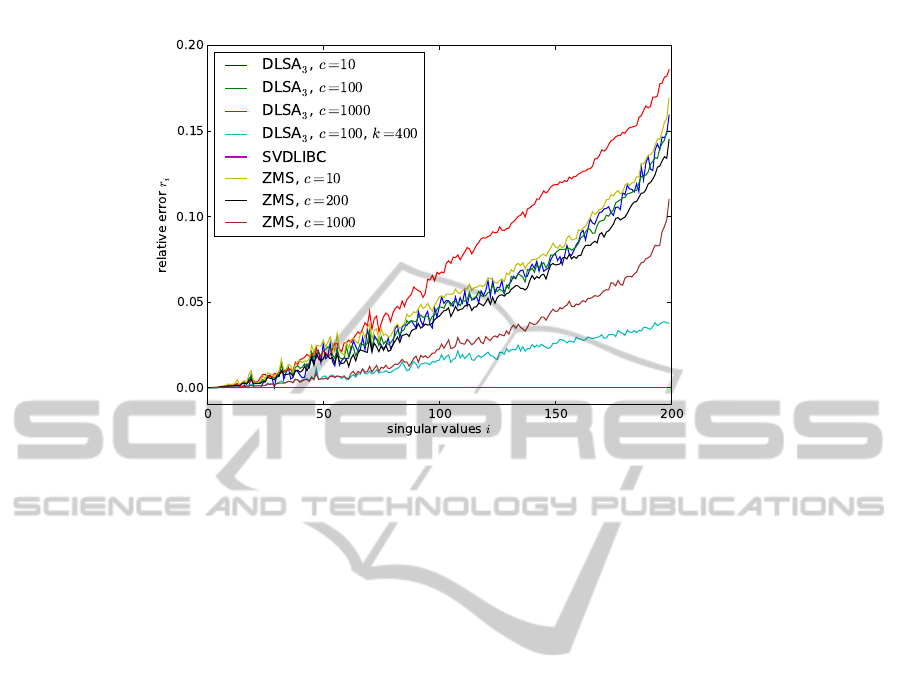
Figure 1: Accuracy of singular values for various decomposition algorithms.
This method is suited for processing extremely
large (possibly infinite) sparse matrices that arrive as a
stream of observations, where each observation must
be immediately processed and then discarded. It is
therefore best suitable for environments where the in-
put stream cannot be repeated and must be processed
in constant memory.
Future work will include a more thorough eval-
uation of the algorithm’s accuracy and performance,
with a side-by-side comparison to other decomposi-
tion algorithms.
ACKNOWLEDGEMENTS
This study was partially supported by the LC536
grant of MMT CR.
REFERENCES
Berry, M. (1992). Large-scale sparse singular value compu-
tations. The International Journal of Supercomputer
Applications, 6(1):13–49.
Brand, M. (2006). Fast low-rank modifications of the thin
singular value decomposition. Linear Algebra and its
Applications, 415(1):20–30.
Comon, P. and Golub, G. (1990). Tracking a few extreme
singular values and vectors in signal processing. Pro-
ceedings of the IEEE, 78(8):1327–1343.
Deerwester, S., Dumais, S., Furnas, G., Landauer, T., and
Harshman, R. (1990). Indexing by Latent Semantic
Analysis. Journal of the American society for infor-
mation science, 41(6):391–407.
ehek, R. and Sojka, P. (2010). Software Framework for
Topic Modelling with Large Corpora. In Proceedings
of LREC 2010 workshop on New Challenges for NLP
Frameworks, pages 45–50.
Golub, G. and Van Loan, C. (1996). Matrix computations.
Johns Hopkins University Press.
Levy, A. and Lindenbaum, M. (2000). Sequential
Karhunen–Loeve basis extraction and its application
to images. IEEE Transactions on Image processing,
9(8):1371.
Salton, G. (1989). Automatic text processing: the transfor-
mation, analysis, and retrieval of information by com-
puter. Addison-Wesley Longman Publishing Co., Inc.
Boston, MA, USA.
Vigna, S. (2008). Distributed, large-scale latent semantic
analysis by index interpolation. In Proceedings of the
3rd international conference on Scalable information
systems, pages 1–10. ICST.
Zha, H., Marques, O., and Simon, H. (1998). Large-scale
SVD and subspace-based methods for Information
Retrieval. Solving Irregularly Structured Problems in
Parallel, pages 29–42.
Zha, H. and Simon, H. (1999). On updating problems in
Latent Semantic Indexing. SIAM Journal on Scientific
Computing, 21:782.
Zha, H. and Zhang, Z. (2000). Matrices with low-rank-
plus-shift structure: Partial SVD and Latent Semantic
Indexing. SIAM Journal on Matrix Analysis and Ap-
plications, 21:522.
SPEEDING UP LATENT SEMANTIC ANALYSIS - A Streamed Distributed Algorithm for SVD Updates
451
