AN APPROACH TO SEMI-SUPERVISED CLASSIFICATION USING

THE HUNGARIAN ALGORITHM

Amparo Albalate, Aparna Suchindranath and Wolfgang Minker

Institute of Information Technology, University of Ulm, Ulm, Germany

Keywords:

Semi-supervised classiﬁcation, Clustering, Hungarian algorithm, Cluster pruning.

Abstract:

In this paper we propose a novel semi-supervised classiﬁcation algorithm from the cluster-and-label frame-

work. A small amount of labeled examples is used to automatically label the extracted clusters, so that the

initial labeled seed is implicitely ”augmented” to the whole clustered data. The optimum cluster labelling is

achieved by means of the Hungarian algorithm, traditionally used to solve any optimisation assignment prob-

lem. Finally, the augmented labeled set is applied to train a SVM classiﬁer. This semi-supervised approach

has been compared to a fully supervised version. In our experiments we used an artiﬁcial dataset (mixture

of Gaussians) as well as other ﬁve real data sets from the UCI repository. In general, the experimental re-

sults showed signiﬁcant improvements in the classiﬁcation performance under minimal labeled sets using the

semi-supervised algorithm.

1 INTRODUCTION

Semi-supervised classiﬁcation is a framework of al-

gorithms proposed to improve the performance of su-

pervised algorithms through the use of both labeled

and unlabeled data (Design et al., ). One reported lim-

itation of supervised techniques is their requisite of

available training corpora of considerable dimensions

order to achieve accurate predictions on the test data.

Furthermore, the high effort and cost associated to la-

beling large amount of training samples by hand -a

typical example is the manual compilation of labeled

text documents- is a second limiting factor, which led

to the development of semi-supervised techniques. It

has been shown in numerous studies how the knowl-

edge learned from unlabeled data can dramatically re-

duce the size of labeled data required to achieve ap-

propriate classiﬁcation performances (Nigam et al.,

2000; Castelli and Cover, 1995).

Different approaches to semi-supervised classiﬁ-

cation have been proposed in the literature, including,

among others, Co-training (Maeireizo et al., 2004),

self-training (Yarowsky, 1995) or generative models

(Nigam et al., 2000; Dempster et al., 1977). Two ex-

tensive surveys on semi-supervised learning are pro-

vided in (Zhu, 2006) and (Seeger, 2001). This pa-

per focuses in a particular case of generative mod-

els, in which cluster algorithms are employed instead

of probabilistic mixture models. This kind of ap-

proaches is commonly referred to as “cluster-and-

label” framework (Zhu, 2006). The algorithm pro-

posed in this paper differs from previous works in

which both clustering and labeling stages are often

integrated in one single process. Previously, the la-

beled seeds have been often used to initialise or guide

the clustering algorithms, in such a way that the clus-

ters’ patterns are implicitely tagged during the clus-

tering process (Demiriz et al., 1999). In this work,

however, the clustering and labeling tasks are sepa-

rated into two independent processes. First, a cluster

partition of the data set is obtained through a fully un-

supervised clustering algorithm. Then, given a small

set of labels (also referred to as prototype of labeled

seed), a cost matrix is computed based on the distri-

bution of labels through the clusters. The cluster la-

beling objective is then formulated as an assignment

problem, which has been solved using the Hungarian

algorithm (Kuhn, 1955). Thereby, an optimum clus-

ter labeling given the labeled seeds is ensured. An

extension of the proposed semi-supervised approach

is also presented, using a cluster-pruning algorithm

which is intended to improve the quality of the clus-

ters by pruning such patterns with high probability of

belonging to a overlapping region between classes.

The paper is organised as follows: Section 2 pro-

vides an overview of related work in the ﬁeld semi-

supervised classiﬁcation. In Section 3, we outline the

proposed algorithm. One important task in the new

424

Albalate A., Suchindranath A. and Minker W..

AN APPROACH TO SEMI-SUPERVISED CLASSIFICATION USING THE HUNGARIAN ALGORITHM.

DOI: 10.5220/0003187304240433

In Proceedings of the 3rd International Conference on Agents and Artiﬁcial Intelligence (ICAART-2011), pages 424-433

ISBN: 978-989-8425-40-9

 2011 SCITEPRESS (Science and Technology Publications, Lda.)

algorithm is the optimum cluster labeling, which is

explained in more detail in Section 4. In Section 5

we propose an extension to the semi-supervised algo-

rithm described in Section 3. The data sets used in

the experiments are introduced in Section 6. Finally,

we draw conclusions and future directions algorithm

in Section 7.

2 RELATED WORK

Different types of semi-supervised classiﬁers can be

distinguished in the literature. Among them, in this

section we brieﬂy describe three of the main ap-

proaches: self-training, co-training and generative

models.

2.1 Self-training

In self training, a single classiﬁer is iteratively trained

with a growing set of labeled data, starting from a

small initial seed of labeled samples. Commonly, an

iteration of the algorithm entails the following steps:

1) training on the labeled data available from previ-

ous iterations, 2) Applying the model learned from la-

beled data to predict the unlabeled data and 3) Sorting

the predicted samples according to their conﬁdence

scores and adding the top most conﬁdent ones with

their predicted labels to the labeled set.

One example of self training is the work by

Yarowski (Yarowsky, 1995) on word sense disam-

biguation. A self training approach was applied to to

classify a word and its context into the possible word

senses in a polysemic corpus, starting by a tagged

seed for each possible sense of the words.

2.2 Co-training

In a similar way as self-training, co-training ap-

proaches are based on an incremental augmentation

of the labeled seeds by iteratively classifying the unla-

beled sets and attaching the most conﬁdent predicted

samples to the labeled set. However, in contrast to

self training, two complementary classiﬁers are si-

multaneously applied, fed with two different “views”

of the feature set. The prediction of the ﬁrst classi-

ﬁer is used to augment the labeled set available to the

second classiﬁer and vice-versa. In (Maeireizo et al.,

2004), a co-training strategy was applied to predict

the emotional/non-emotional character of a corpus

of student utterances collected within the ITSPOKE

project (Intelligent Tutoring Spoken dialog system).

The authors selected two high-precision classiﬁers.

The ﬁrst one was trained to recognise the emotional

status of an utterance (e.g. ’1’ emotional vs ’0’ for

non-emotional), while the second one predicted its

non-emotional status (’1’ non-emotional vs. ’0’ emo-

tional). The labeled set was iteratively increased by

attaching the top most conﬁdent predicted samples to

the labeled set from previous iterations.

2.3 Generative Models

Given a data set of observations X , with the corre-

sponding set of class labels, Y , a generative model

assumes that the observations and labels are drawn

according to a model p(x, y) whose parameters should

be “identiﬁable” (Zhu, 2006). Typically, the Expecta-

tion Maximisation algorithm is applied to estimate the

model parameters (Nigam et al., 2000).

Other strategies attempt to derive the underlying

class distribution by means of clustering techniques.

These approaches are commonly referred to as the

cluster -and- label paradigm. For example, in (Demi-

riz et al., 1999) a genetic k-means clustering was im-

plemented using a genetic algorithm. The goal of the

algorithm was to ﬁnd a set of k cluster centres that

simultaneously optimised an internal quality objec-

tive (e.g minimum cluster dispersion) and an exter-

nal criterion based on the available labels (e.g mini-

mum cluster entropy). The simultaneous optimisation

concerning internal and external criteria was attained

through the formulation of a new objective function

as a linear combination of both criteria.

3 NOVEL SEMI-SUPERVISED

ALGORITHM USING THE

CLUSTER AND LABEL

STRATEGY

In this paper we propose a new semi-supervised al-

gorithm, according to a cluster-and-label strategy. As

explained in Section 1, in previous works, the label-

ing task has been often integrated into the clustering

process as a simultaneous optimisation problem. In

other words, the clusters’ patterns are simultaneously

tagged during the clustering process.

Such simultaneous deﬁnition of the optimisation

problem (clustering/labeling) produces a certain de-

pendency of the extracted clusters with respect to the

initial labels. Thus, potential labeling errors present

in the labeled seeds may also induce a certain degra-

dation of the clustering solution. In fact, training sets

are not exempt from potential labeling errors. These

may occur depending on the degree of expertise of the

human annotators. Even for expert labelers, the con-

AN APPROACH TO SEMI-SUPERVISED CLASSIFICATION USING THE HUNGARIAN ALGORITHM

425

ﬁdence in annotating patterns with a certain degree

of ambiguity may drop down signiﬁcantly, as it hap-

pens, for example, with the annotation of non-acted

emotions.

In other to avoid the aforementioned limitation,

the approach proposed in this paper distinguishes the

clustering and labeling processes as two indepen-

dent optimisation problems. Essentially, the data set

(both labeled and unlabeled patterns) is ﬁrst clustered,

without any a-priory information concerning labels.

Thereby, a fully unsupervised, data-driven solution

is enforced which optimises an internal quality ob-

jective. Then, the distribution of labels through the

different clusters is taken into consideration in order

to achieve the optimum labeling of the clusters’ pat-

terns. Thereby, higher robustness against possible er-

rors in the labeled seeds is achieved in the proposed

approach.

Data Set. First, the data is divided into a test set

(∼ 10%) and a training set ( ∼ 90%). Let

= {x

, x

, ··· , x

}, ∀x

∈ R

denote the training data points. This set is in turn

divided by two disjoint subsets:

= X

(l)

∪ X

(u)

denoting X

(l)

the labeled portion of X

for which

the corresponding set of labels Y

is assumed to be

known, and X

(u)

, the subset of unlabeled patterns in

Clustering. The ﬁrst step in the semi-supervised

approach is to ﬁnd a cluster partition C of the train-

ing data X

in to a set of k disjoint clusters C =

, . . . ,C

}, where k is the number of classes

(which is assumed to be known from the labeled

set). In this work, the Partitioning around Medoids

(Pam) algorithm has been selected using the Eu-

clidean distance to compute dissimilarity matrices.

The Pam clustering algorithm provides the cluster so-

lution wich minimises the sum of distances to the

cluster medoids.

Optimum Cluster Labeling. The labeling block

performs a crucial task in the semi-supervised

algorithm. Given the set of clusters C in which the

training data is divided, the objective of this block

is to ﬁnd an optimum bijective mapping of labels to

clusters:

L : C → K , K = {1, 2, 3, ·· · , k}

so that an optimum criterion is fulﬁlled. Each

cluster is assigned exactly one class label in K . This

mapping of clusters to class labels is equivalent to a

mapping function that assigns, to each clustered pat-

tern, the class label of the cluster where it belongs.

As a result of cluster labeling, the initial labeled seed

(l)

, Y

(l)

) is extended to the complete training set

, Y

), denoting Y

, the set of augmented labels

corresponding to the observations in X

Classiﬁcation. Finally, a Support Vector Machine

(SVM) classiﬁer (Burges, 1998; Joachims et al.,

1997) is trained with the augmented labeled set

, Y

) obtained after cluster labeling. The SVM

learned model is then applied to predict the labels for

the test set.

Simultaneously, a fully supervised classiﬁcation

scheme has been compared to the semi-supervised al-

gorithm. In this case, the SVM is directly trained with

the initial labeled seed (X

(l)

, Y

(l)

Both semi-supervised and supervised strategies

have been evaluated in terms of accuracy, by compar-

ing the predicted labels of the test patterns with their

respective manual labels. The evaluation results are

discussed in Section 6.

4 OPTIMUM CLUSTER

LABELING

In this section, we described in more detail optimum

cluster labeling task in the proposed semi-supervised

algorithm.

Problem Deﬁnition. Given the training data,

= X

(l)

∪ X

(u)

, the set Y

(l)

of labels associated to

the portion X

(l)

of the training set, the set K of labels

for the k existing classes

, and a cluster partition C of

into disjoint clusters, the optimum cluster label-

ing problem is to ﬁnd a bijective mapping function, L:

L : C → K , K = {1, 2, 3, · · · , k}

that assigns each cluster in C to a class label in K ,

while minimising the total labeling cost. This cost is

deﬁned in terms of the labeled seed (X

(l)

, Y

(l)

) and

the set of clusters C . Consider the following matrix

of overlapping products N:

Although class labels can take any arbitrary value, ei-

ther numeric or nominal, for simplicity in the formulation

and implementation of the cluster labeling problem the k

class labels are transformed to integer values ([1. . . k]).

ICAART 2011 - 3rd International Conference on Agents and Artificial Intelligence

426

N =







··· n







with constituents n

, denoting the number of la-

beled patterns from X

(l)

with class label y = i that fall

into cluster C

. The labeling objective is to minimise

the global cost of the cluster labeling denoted by L:

Total Cost(L) =

∑

∈C

·Cost



L(C

)



(1)

where W = (w

, ··· , w

) is a vector of weights for

the different clusters. For example, it may be used if

clusters sizes show signiﬁcant differences among the

clusters. In this paper, the weights are assumed to be

equal for all clusters, so that w

= 1, ∀i ∈ 1··· k.

The individual of labeling a cluster C

with class j is

deﬁned as the number of samples from class j (in the

labeled seed) that fall outside the cluster C

, i.e.:

Cost



L(C

)



∑

6=C

L(C

),k

(2)

by applying Equation 2 into the total cost deﬁni-

tion of Equation 1, yields:

Total Cost(L) =

∑

∈C

∑

6=C

L(C

),k

(3)

Using a greedy search algorithm, the cost minimi-

sation of Equation 1 requires k! operations (where

k denotes the number of clusters/classes). Such a

complexity becomes computationally intractable for

k ≥ 10. However, larger number of classes are often

involved in real classiﬁcation problems. In this pa-

per, the Hungarian algorithm have been used, which

can achieve the optimum cluster labeling with sub-

stantially lower complexities. It requires the def-

inition of a cost matrix C

[kxk]

, whose rows denote

the clusters and the columns are referred to class la-

bels in K . The elements C

denote the individual

costs of assigning the cluster C

to class label j, i.e.

= Cost(L(C

) = j).

4.1 The Hungarian Algorithm

The hungarian algorithm was devised by Harold

Huhn in 1955 to solve the optimum assignment prob-

lem in polynomial time. The name “Hungarian” was

given after two hungarian scientists who had previ-

ously established large part of the algorithm’s mathe-

matical background. It ﬁnds the optimum assignment

on a matrix of costs where each element C

i, j

denotes

the penalty paid for the corresponding individual as-

signment (i, j). A typical example is the worker-job

assignment where the rows represent different work-

ers and the columns are the jobs to which the workers

can be designated to. The original algorithm proposed

by Huhn solved the assignment task in O(k

) opera-

tions, although some extensions of the algorithm have

been proposed, leading to a complexity of O(k

The Hungarian algorithm has been described in

terms of bipartite graphs, or equivalently, as a number

of steps involving certain manipulations of the input

cost matrix, which can be summarised as follows.

1. Substract from each row of the cost matrix, the

values of the smallest element in the row.

2. Proceed as in step 1. columnwise.

3. Cross out the necessary rows and/or columns to

cover all zeros in the modiﬁed cost matrix from

step 2. by drawing the minimum number of lines.

4. If a number of k lines have been drawn, proceed

to perform the assignments in step 5. Otherwise

select the smallest number not covered by any

line drawn in step 3. Substract this value to the

non-covered elements, adding the value to the el-

ements that are covered by two lines.

5. Starting from the ﬁrst row, if the row contains a

unique zero element in a column j, assign the

worker in the row to the j

job. Prune the row and

column from the cost matrix and continue scan-

ning the rest of rows. If some of the assignments

are still left at the end of this process, repeat the

procedure columnwise. If still some assignments

are left, it means that a unique assignment is not

possible. In such case, the remaining assignments

can be performed at random.

5 DATA SETS

Mixture of Gaussians. This data set comprises a

mixture seven Gaussians in two dimensions and 1750

instances (250 in each Gaussian), where a certain

amount of overlapping patterns (potential ambigui-

ties) can be observed.

Iris Data Set (Iris). The Iris set is one of the most

popular datasets from the UCI repository (uci, ). It

comprises 150 instances iris of 3 different classes of

iris ﬂowers (Setosa, Versicolor, virginica). Two of

these classes are linearly separable while the third one

is not linearly separable from the second one.

AN APPROACH TO SEMI-SUPERVISED CLASSIFICATION USING THE HUNGARIAN ALGORITHM

427

Wine Data Set (Wine). The wine set is one of the

popular data sets from the UCI repository. It consists

of 178 instances with 13 attributes, representing three

different types of wines.

Wisconsin Breast Cancer Data Set (Breast). This

data set constains 569 instances in 10 dimensions, de-

noting 10 different features extracted from digitised

images of breast masses. The two existing classes are

referred to the possible breast cancer diagnosis (ma-

lignant, benign).

Handwritten Digits Data Set (Pendig). The fourth

real data set is for pen-based recognition of handwrit-

ten digits. In our experiments, we used the test parti-

tion

, composed of 3498 samples with 16 attributes.

Ten classes can be distinguished for the digits 0-9.

Pima Indians Diabetes (Diabetes). This data set

comprises 768 instances with 8 numeric attributes.

Two classes denote the possible diagnostics (the pa-

tients show or not signs of diabetes.).

6 EXTENSION THROUGH

CLUSTER PRUNING

In this section, an alternative to the cluster-and-label

strategy is introduced. Even though the underlying

class structure can be appropriately captured by a

cluster algorithm, the augmented data set derived by

the optimum cluster labeling may contain a number

of “misclassiﬁcation”

errors with respect to the real

class labels. This happens specially when two or more

of the underlying classes show a certain overlapping

of patterns. In this case, the errors may be accumu-

lated in the regions close to the cluster boundaries of

adjacent clusters.

The general idea behindthe proposed optimisation

method is to improve the (external) cluster quality

by identifying and removing such regions with high

probability of missclassiﬁcation errors from the clus-

ters. To this aim, the concept of pattern silhouettes

has been applied to prune the clusters in C .

The silhouette width of an observation x

is an in-

ternal measure of quality, typically used as the ﬁrst

due to memory limitations of the R software used in the

experiments

The term missclassiﬁcation is not here used to indicate

the predicted errors of the end classiﬁers but the errors after

the cluster labeling block. Note that, after cluster labeling,

each clustered data pattern is assigned a class label (the la-

bel of its cluster), which can be compared to the real label

if the complete labeled set is available.

step for the computation of average silhouette width

of a cluster partition (Rousseeuw, 1987). It is formu-

lated as:

s(x

) =

b(x

) − a(x

)

max(a(x

), b(x

))

(4)

where a is the average distance between x

and the

elements in its own cluster, while b is the smallest

average distance between x

and other clusters in the

partition. Intuitively, the silhouette of an object s(x

can be thought of as the “conﬁdence” to which the

pattern x

has been assigned to the cluster C(x

) by

the clustering algorithm. Higher silhouette scores are

observed for patterns clustered with a higher “con-

ﬁdence”, while low values indicate patterns which

lie between clusters or are probably allocated in the

wrong cluster.

The cluster pruning approach can be described as

follows:

Input A cluster partition C of the data set; the

distance matrix D

Output A set of pruned clusters C

′

1. Given a cluster partition C and the matrix of

dissimilarities between the patterns in the data set, D,

calculate the silhouette of each object in the data set.

2. Sort the elements in each cluster according to their

silhouette scores, in increasing order.

3. In each cluster, the elements with high silhouettes

can be considered as objects with high “clustering

conﬁdence”. In contrast, such elements with low

silhouette values are clustered with lower conﬁdence.

This latter kind of objects may thus belong to a

class-overlapping region with higher probability.

Using the histograms of silhouette scores within the

clusters, select a minimum silhouette threshold for

each cluster. Further details about the selection of

silhouette thresholds by the cluster pruning algorithm

are provided in Section 6.1.

4. Prune each cluster C

in C by removing patterns

which do not exceed the minimum silhouette thresh-

old for the cluster, chosen in the previous step.

6.1 Determination of Silhouette

Thresholds

In the proposed cluster pruning method, different sil-

houette thresholds are applied according to the dis-

tribution of silhouette values within each cluster, es-

ICAART 2011 - 3rd International Conference on Agents and Artificial Intelligence

428

timated through histograms. Assuming that the un-

derlying class distribution is appropriately captured in

the cluster partition, if a signiﬁcant distortion of the

original clusters is introduced through cluster prun-

ing, the learned SVM models may also deviate from

the expected models to a certain extent. The objec-

tive is to remove potential clustering errors while pre-

serving to the highest possible extent the shape and

size of the original clusters. In practice, pruning an

amount of patterns from 20% to 30% of the cluster

size has been considered appropriate for the current

purpose. In addition, the selected thresholds also de-

pend on the pattern silhouette values: patterns with a

silhouette score larger than 0.5 are deemed to be clus-

tered with a sufﬁciently high “conﬁdence”. Thus, the

maximum silhouette threshold applied in the cluster

pruning algorithm is sil

= 0.5. In consequence, if

the minimum observed silhouette score in a cluster is

larger than 0.5, the cluster remains unaltered in the

pruned partitions.

The speciﬁc criteria to select the silhouette thresh-

olds can illustrated by considering the clusters ex-

tracted from the Breast data set (all 569 data in-

stances). The distribution of silhouette scores has

been estimated by using the histogram function in

the R-software, which also provides the vectors of

silhouette values found as the histogram bin limits

and the counts of occurrences in each bin

. The

silhouette thresholds have been selected to coincide

to histogram bin limits’. In the Breast data set (2

classes/clusters), the vector of silhouette thresholds

for the ﬁrst and second clusters is [0.5, 0.2]. The value

sil

= 0.5 for the ﬁrst cluster corresponds to the up-

per bound for the silhouette thresholds, as explained

in the previous paragraph. It results in the removal of

5.2% of the cluster’s patterns. For the second clus-

ter, the threshold sil

= 0.2 is selected. The pruned

section associated to sil

corresponds to the ﬁrst ﬁve

histogram bins, comprising 25% of the patterns in the

cluster. By including the sixth histogram bin in the

pruned section, the next possible silhouette thresh-

old level is sil

= 0.3, However, such threshold level

would lead to the removal of a considerable amount

(46.28%) of the cluster patterns, which is considered

unacceptable for preserving the cluster size/shape.

To summarise, the number of histogram bins cor-

responding to rejected patterns is determined accord-

ing to one of these two conditions: (1) the upper limit

of the last rejected bin should not be greater than

sil

= 0.5, and (2) The amount of rejected patterns

(total number of occurrences in the rejected bins)

The bin sizes provided by the R-software histogram

function are estimated according to the Sturges formula

(Freedman and Diaconis, 1981)

should not exceed a ratio of 30% of the total number

of patterns in the cluster.

6.2 Evaluation of the Cluster Pruning

Approach

In this section, the efﬁciency of the cluster pruning

method for rejecting missclassiﬁcation errors from

the clustered data is evaluated through an analysis of

the algorithm outcomes on the Iris, Wine, Breast Can-

cer, Diabetes, Pendig and Seven Gaussians data set

For the purpose of evaluating the cluster prun-

ing algorithm, the cluster labeling task has been per-

formed using the complete set of labels for each data

set. The resulting misclassiﬁcation error rates as well

as the NMI results observed in Table 1 conﬁrm the

adequate behaviour of the proposed cluster pruning

algorithm for removing such sections from the clus-

ters with high probability of resulting in misclassi-

ﬁcation errors after cluster labeling. For instance,

while the pruned sections comprise around 10− 20%

of the patterns in the data sets, the percentage of

remaining misclassiﬁcation errors has been substan-

tially reduced. As an example, the error rate has

dropped from 10.66% to 4.03% after pruning on the

Iris data set, while error rates have been reduced from

4.09% to 0.99% for the Breast data set, and from

22.40% to 8.98% in the Wine dataset. An exception

to the previous observations is the Diabetes data set,

in which the error rate after cluster pruning (38.16%)

remains very similar to the original missclassiﬁcation

rate (40.10%) - note that, for 2 clusters as in the case

of the Diabetes data, the worst possible error rate that

can be observed is of 50%. Any error rate larger than

50% is not observed as it just produces an inversion of

the cluster labels. In other words, the original error in

the diabetes data set implies almost a roughly uniform

distribution of patterns from any of the two underly-

ing classes in the extracted clusters. This fact is also

evidenced by the NMI score 0.012. In consequence,

the error rate is roughly the same after cluster prun-

ing, and the removal of patterns by means of cluster

pruning algorithm is just as efﬁcient as removing the

same amount of patterns at random.

7 SIMULATIONS AND RESULTS

In the experimental setting, SVMs have been used as

the baseline classiﬁer. First, each data set has been

note that the cluster partitions obtained in this experi-

ments comprise all instances of the data sets (without prior

partitions into test/training).

AN APPROACH TO SEMI-SUPERVISED CLASSIFICATION USING THE HUNGARIAN ALGORITHM

429

Table 1: Some details about the cluster pruning approach in the Iris, Wine, Breast cancer, Diabetes, pendig and Seven

Gaussians data set.

Data Set

Silhouette % Removed

Error 1 (%) Error 2 (%) NMI 1 NMI 2

thresholds patterns

Iris [0.5 0.3 0.4] 17.33% 10.66 % 4.03% 0.758 0.888

Wine [0.2 0.14 0.24] 22.40 % 8.98 % 0.72% 0.783 0.967

Breast [0.5 0.2] 11.56 % 4.09 % 0.99% 0.741 0.910

Diabetes [0.5 0.1] 16.35 % 40.10% 38.16% 0.012 0.022

[0.2 0.3 0.2 0.2

Pendig 0.25 0.2 0.15 0.15 20.10 % 31.93% 21.22% 0.701 0.796

0.25 0.2]

Seven [0.4 0.5 0.4 0.4

Gaussians 0.4 0.4 0.4] 11.77 % 0.27% % 0.02% 0.944 0.993

divided into two training (∼ 90%) and test (∼ 10%)

subsets. In order to avoid possible biases of a single

test set or labeled seed, such partition of the data set

into a training and test portions has been randomly

repeated to generate 20 different partitions. Also,

for each one of these partitions, 20 different random

seeds of labeled prototypes (n labels /category) have

been selected. In total, 400 different prototype seeds

(20x20) have been obtained. In the experiments, only

prototype labels are assumed to be known a-priory.

No other class label knowledge has been applied to

any of the algorithm stages. Each prototype seed has

been used as the availabe training set for the super-

vised SVM. In the semi-supervised approach, these

labeled prototype seeds have been used to trigger the

automatic cluster labeling.

Both supervised and semi-supervised SVM clas-

siﬁers have been evaluated on an accuracy basis, con-

sidering different number of labeled prototypes (sam-

ples) per category, from n = 1 to n

max

= 30. The ac-

curacy results obtained on the different data sets are

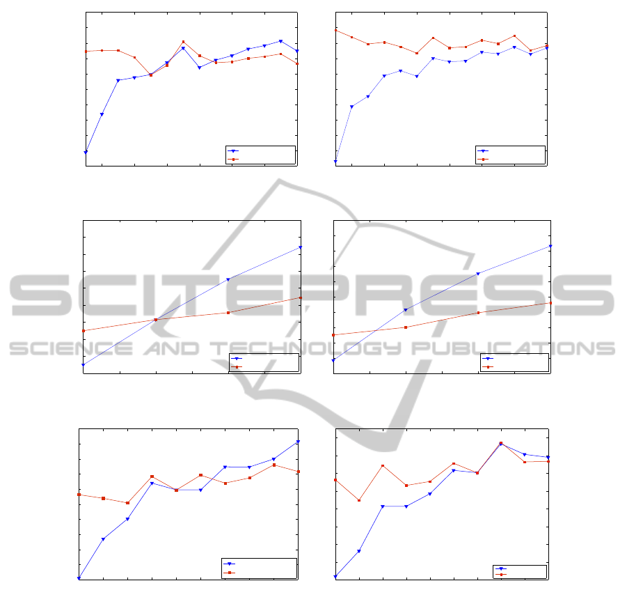
shown in Figures 1 and 2. In particular, left plots are

referred to the supervised and the semi-supervised ap-

proach without cluster pruning, while right plots are

referred to the semi-supervised approaches by incor-

porating the cluster pruning approach.

Note that the right and left plots are obtained from

different experiments (in each experiment a differ-

ent labeled seed is involved) so that the mean ac-

curacy values of the supervised approach in left and

right plots can slightly differ. In all cases, horizontal

axes are referred to the sizes of the initial prototype

seeds, whereas vertical axes indicate the mean accu-

racy scores, averaged over the 400 prototype initiali-

sations.

As it can be observed in Figures 1 and 2, the mean

accuracy curves of the semi-supervised algorithm are

roughly constant or slowly increasing with the labeled

set size. Certain random variations can be observed,

since the experiment outcomes for different seed sizes

are referred to different random prototype seeds (note,

however, that for each labeled set size, both super-

vised and semi-supervised outcomes have been simul-

taneously obtained with identical sets of prototypes,

so that their respective accuracy curves can be com-

pared). In contrast, accuracy curves of the supervised

approach show stronger increasing trends with the la-

beled set sizes. In the Seven Gaussians, Iris, Pendig,

Wine and Breast Cancer data sets, the mean accuracy

curves for the supervised and semi-supervised algo-

rithms intersect at certain labeled set sizes, n

′

. For

smaller labeled seed sizes (n< n

′

), the training “infor-

mation” available in the augmented labeled sets (af-

ter cluster labeling) is clearly superior than the the

small labeled seeds. Therefore, although the aug-

mented labels are not exempt from misclassiﬁcations

due to clustering errors, higher prediction accuracies

are achieved by the semi-supervised approach with re-

spect to the supervised classiﬁer. For (n ≥ n

′

), the

information in the increasing labeled seeds compen-

sates for the missclassiﬁcation errors present in the

augmented sets and thus the supervised classiﬁer out-

performs the semi-supervised approach. As shown in

the previous section, these errors present in the aug-

mented data sets can be notably reduced by means

of cluster pruning. In consequence, an improvement

in the prediction accuracies achieved by the semi-

supervised algorithm is generally observed by incor-

porating the cluster-pruning algorithm. Note that the

values of n shown in the plots range from n = 0 to

values slightly larger than the respective intersection

points n

′

Unlike the accuracy results observed in the Seven

Gaussians, Iris, Pendig, Wine and Breast Cancer data

sets, a degradation in the semi-supervised classiﬁca-

tion performance with respect to the supervised clas-

siﬁer is observed in the Diabetes data set, regard-

less of the initial labeled seed sizes. This observa-

ICAART 2011 - 3rd International Conference on Agents and Artificial Intelligence

430

2 4 6 8 10 20 30

0.935

0.94

0.945

0.95

0.955

0.96

0.965

0.97

0.975

0.98

0.985

Number of labeled patterns/category

Accuracy

Seven Gaussians data set

SVM

Semi−supervised

(a)

2 4 6 8 10 20 30

0.935

0.94

0.945

0.95

0.955

0.96

0.965

0.97

0.975

0.98

0.985

Number of labeled patterns/category

Accuracy

Seven Gaussians data set (pruned clusters)

SVM

Semi−supervised

(b)

1 1.5 2 2.5 3 3.5 4

0.66

0.68

0.7

0.72

0.74

0.76

0.78

0.8

0.82

0.84

Number of labeled patterns/category

Accuracy

Pendig data set

SVM

Semi−supervised

(c)

1 1.5 2 2.5 3 3.5 4

0.64

0.66

0.68

0.7

0.72

0.74

0.76

0.78

0.8

0.82

0.84

Number of labeled patterns/category

Accuracy

Pendig data set (pruned clusters)

SVM

semi−supervised

(d)

1 2 3 4 5 6 7 8 9 10

number of labelled patterns/class

% accuracy

Iris data set

SVM

Semi−supervised

(e)

1 2 3 4 5 6 7 8 9 10

0.78

0.8

0.82

0.84

0.86

0.88

0.9

0.92

0.94

Number of labeled patterns/class

Accuracy

IRIS data set (pruned clusters)

SVM

Semi−supervised

(f)

Figure 1: Mean accuracy curves obtain by the supervised (blue curves) and semi-supervised (red curves)classiﬁers. Left plots

are referred to the basic semi-supervised approach, while right plots are obtained with the extension of the semi-supervised

approach by means of cluster pruning.

tion is strictly associated to the NMI scores of the

extracted clusters presented in the previous section

(NMI=0.012), which corresponds to a missclassiﬁca-

tion rate of 40.10%. This means that almost no infor-

mation concerning class labels is present in the aug-

mented data sets used to train the SVM models. As a

consequence, the semi-supervised performanceon the

diabetes data set is thus comparable to the a classiﬁer

which just performs random predictions, as it corre-

sponds to the use of “unlabeled data alone” (Castelli

and Cover, 1995).

8 CONCLUSIONS AND FUTURE

DIRECTIONS

In this paper, a semi-supervised approach has been

presented based on the cluster-and-label paradigm.

In contrast to previous works in the semi-supervised

classiﬁcation literature, in which labels are commonly

integrated in the clustering process, in this work,

the cluster and labeling processes are independent

from each other. First, a conventional unsupervised

clustering algorithm, the partitioning around medoids

AN APPROACH TO SEMI-SUPERVISED CLASSIFICATION USING THE HUNGARIAN ALGORITHM

431

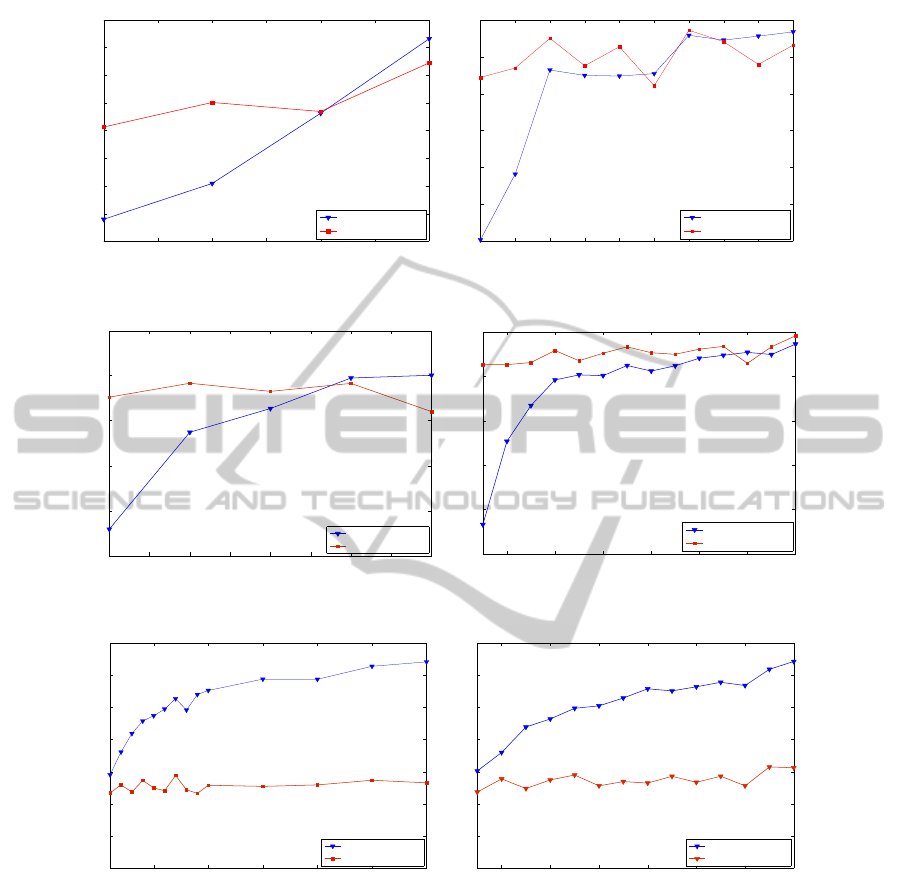
1 1.5 2 2.5 3 3.5 4

Breast Cancer data set

number of labelled patterns/class

% accuracy

SVM

Semi−supervised

(a)

1 2 3 4 5 6 7 8 9 10

0.91

0.92

0.93

0.94

0.95

0.96

0.97

Number of labeled pattens/class

Accuracy

Breast Cancer data set (pruned clusters)

SVM

Semi−supervised

(b)

1 1.5 2 2.5 3 3.5 4 4.5 5

100

Number of labelled patterns/class

% accuracy

Wine data set

SVM

Semi−supervised

(c)

2 4 6 8 10 20 30

0.75

0.8

0.85

0.9

0.95

Number of labeled patterns/class

Accuracy

WINE data set (pruned clusters)

SVM

Semi−supervised

(d)

5 10 15 20 25 30

0.4

0.45

0.5

0.55

0.6

0.65

0.7

0.75

number of labeled patterns/class

% accuracy

Diabetes Data set

SVM

Semi−supervised

(e)

2 4 6 8 10 20 30

0.4

0.45

0.5

0.55

0.6

0.65

0.7

0.75

Number of labeled patterns/category

Accuracy

Diabetes data set (pruned clusters)

SVM

Semi−supervised

(f)

Figure 2: Mean accuracy curves obtain by the supervised (blue curves) and semi-supervised (red curves)classiﬁers.

(PAM) (Kaufmann and Rousseeuw, 1990) is used to

obtain a cluster partition. Then, the output cluster par-

tition, as well a small set of labeled prototypes (also

referred to as labeled seeds) are used to decide the op-

timum cluster labeling given the labeled seed. The

cluster labelling problem has been formulated as a

typical assingment optimisation problem, whose so-

lution is obtained by means of the Hungarian algo-

rithm. Experimental results have shown signiﬁcant

improvements in the classiﬁcation accuracy for mini-

mum labeled sets, in such data sets where the under-

lying classes can be appropriately captured by means

of unsupervised clustering.

In addition, an optimisation of the semi-

supervised algorithm has been also developed by dis-

carding the patterns clustered with small silhouette

scores. Thereby, it has been shown that the quality

of the pruned clusters can be improved, as signiﬁcant

reductions of the missclassiﬁcation errors present in

the clustered data are achieved through the removal

of relatively small amounts of patterns from the clus-

ters.

Future work is to investigate other possible alter-

nativesfor the deﬁnition of the cost matrix used by the

ICAART 2011 - 3rd International Conference on Agents and Artificial Intelligence

432

Hungarian algorithm. For example, probabilistic def-

inition of the cost matrix by estimating class-cluster

probabilities given the labeled seeds.

A further issue to be analysed is the choice of the

number of clusters k, to be larger than the number

of predeﬁned categories. We believe such an strat-

egy may provide better classiﬁcation performances -

specially for larger numbers of categories - as clus-

ters can be more “speciﬁed” (lower Entropy values)

with members of one category. In such case, the clus-

ter sizes should be also taken into account for the

deﬁnition of labeling costs. Moreover, this strategy

would result in rectangular (non-square) cost matri-

ces for which the Hungarian algorithm does not apply.

A suitable alternative would be to solve the labeling

problem given the cost matrices by means of genetic

algorithms.

REFERENCES

http://archive.ics.uci.edu.

Burges, C. J. C. (1998). A tutorial on support vector

machines for pattern recognition. Data Mining and

Knowledge Discovery, 2:121–167.

Castelli, V. and Cover, T. M. (1995). On the exponen-

tial value of labeled samples. Pattern Recogn. Lett.,

16(1):105–111.

Demiriz, A., Bennett, K., and Embrechts, M. J. (1999).

Semi-supervised clustering using genetic algorithms.

In In Artiﬁcial Neural Networks in Engineering

(ANNIE-99, pages 809–814.

Dempster, A. P., Laird, N. M., and Rubin, D. B. (1977).

Maximum likelihood from incomplete data via the em

algorithm. Journal of the Royal Statistical Society, Se-

ries B, 39(1):1–38.

Design, I. T., Gabrys, B., and Petrakieva, L. Combining

labelled and unlabelled data.

Freedman, D. and Diaconis, P. (1981). On the histogram as

a density estimator:l2 theory. Probability Theory and

Related Fields, 57(4):453–476.

Joachims, T., Informatik, F., Informatik, F., Informatik, F.,

Informatik, F., and Viii, L. (1997). Text categorization

with support vector machines: Learning with many

relevant features.

Kaufmann, L. and Rousseeuw, P. (1990). Finding Groups

in Data. An Introduction to Cluster Analysis. Wiley,

New York, USA.

Kuhn, H. W. (1955). The hungarian method for the assign-

ment problem. Naval Research Logistics Quarterly,

2:83–97.

Maeireizo, B., Litman, D., and Hwa, R. (2004). Co-training

for predicting emotions with spoken dialogue data. In

Proceedings of the ACL 2004 on Interactive poster

and demonstration sessions.

Nigam, K., McCallum, A. K., Thrun, S., and Mitchell, T.

(2000). Text classiﬁcation from labeled and unlabeled

documents using em. Mach. Learn., 39(2-3):103–134.

Rousseeuw, P. (1987). Silhouettes: A graphical aid to the in-

terpretation and validation of cluster analysis. Jornal

of Computational and Applied Mathematics, 20:53–

65.

Seeger, M. (2001). Learning with labeled and unlabeled

data. Technical report.

Yarowsky, D. (1995). Unsupervised word sense disam-

biguation rivaling supervised methods. In Proceed-

ings of the 33rd annual meeting on Association for

Computational Linguistics.

Zhu, X. (2006). Semi-supervised learning literature survey.

AN APPROACH TO SEMI-SUPERVISED CLASSIFICATION USING THE HUNGARIAN ALGORITHM

433