
IN YOUR INTEREST
Objective Interestingness Measures for a Generative Classifier
Dominik Fisch, Edgar Kalkowski, Bernhard Sick
Computationally Intelligent Systems Lab, University of Applied Sciences Deggendorf, Deggendorf, Germany
Seppo J. Ovaska
Aalto University, School of Science and Technology, Espoo, Finland
Keywords:
Classification, Data mining, Interestingness.
Abstract:
In a wide-spread definition, data mining is termed to be the “non-trivial process of identifying valid, novel,
potentially useful, and ultimately understandable patterns in data”. In real applications, however, usually only
the validity of data mining results is assessed numerically. An important reason is that the other properties are
highly subjective, i.e., they depend on the specific knowledge and requirements of the user. In this article we
define some objective interestingness measures for a specific kind of classifier, a probabilistic classifier based
on a mixture model. These measures assess the informativeness, uniqueness, importance, discrimination,
comprehensibility, and representativity of rules contained in this classifier to support a user in evaluating data
mining results. With some simulation experiments we demonstrate how these measures can be applied.
1 INTRODUCTION
Data mining (DM)—today typically used as a syn-
onym of knowledge discovery in databases (KDD)—
deals with the detection of interesting patterns (e.g.,
regularities) in often huge amounts of data and the
acquisition of knowledge (e.g., classification rules) in
application fields such as marketing, fraud detection,
drug design, and many more. In a well-known defini-
tion, it is termed to be the “non-trivial process of iden-
tifying valid, novel, potentially useful, and ultimately
understandable patterns in data” (Fayyad et al., 1996).
But, how can this “interestingness” of patterns be as-
sessed, in particular numerically? It is obvious that
attributes such as novel, useful, and understandable
are highly subjective as they depend on the particular
needs and the previous knowledge of the data miner.
Thus, usually only the validity of patterns or extracted
knowledge is assessed numerically in order to get an
objective validation of DM results.
In this article, we focus on some other attributes
of data mining results that can be measured numeri-
cally. They are objective on the one hand and related
to attributes such as novelty, usefulness, and under-
standability on the other. For that purpose, we use a
specific classifier, a classifier based on probabilistic
(Gaussian) mixture models (CMM), see also (Fisch
and Sick, 2009; Bishop, 2006). CMM contain rules
that have a form similar to that of fuzzy rules but
they must be interpreted in a probabilistic way. A
rule premise aims at modeling a data cluster in the in-
put space of a classifier, while the conclusion assigns
that cluster to a certain class. Our new interestingness
measures assess the informativeness, uniqueness, im-
portance, discrimination, comprehensibility, and rep-
resentativity of rules contained in a CMM in order to
support a user in evaluating DM results.
In the remainder of the article we briefly discuss
some related work in Section 2. Then, we describe
the classifier and introduce the various interestingness
measures in Section 3. Three case studies in Section
4 show how these measures could be applied. Finally,
we briefly conclude in Section 5 and also give an out-
look to future work.
2 RELATED WORK
Basically, there are subjective and objective interest-
ingness measures that are used to assess rules ex-
tracted from data in a DM process, see, e.g., (Hilder-
man and Hamilton, 2001; McGarry, 2005).
Objective measures are solely based on an anal-
414
Fisch D., Kalkowski E., Sick B. and J. Ovaska S..
IN YOUR INTEREST - Objective Interestingness Measures for a Generative Classifier.
DOI: 10.5220/0003186404140423
In Proceedings of the 3rd International Conference on Agents and Artificial Intelligence (ICAART-2011), pages 414-423
ISBN: 978-989-8425-40-9
Copyright
c
2011 SCITEPRESS (Science and Technology Publications, Lda.)

ysis of the extracted knowledge. These interesting-
ness measures are based, for example, on informa-
tion criteria or on data-based evaluation techniques.
Typical examples are Akaike’s information criterion
or the Bayesian information criterion on the one hand
and statistical measures such as sensitivity, specificity,
precision etc. computed in a cross-validation or a
bootstrapping approach on training/test data on the
other (cf. (Duda et al., 2001; Tan et al., 2004), for
instance). Other criteria that assess the complexity of
rules or rule sets are, e.g., a rule system size measure
(gives the overall number of rules in the rule system),
a computational complexity measure (CPU time re-
quired for the evaluation of a rule or a rule system),
a rule complexity measure (number of attributes that
are tied together in a rule), a mean scoring rules mea-
sure (average number of rules that have to be applied
to come to a conclusion), a fuzzy quality measure (for
terms such as “bad”, “average”, or “very good” that
are associated with rules), the information gain for
association rules (Atzmueller et al., 2004; Taha and
Ghosh, 1997; Nauck, 2003; Hebert and Cremilleux,
2007). Also, measures are combined (e.g., in form
of a weighted sum) in some cases (Atzmueller et al.,
2004; Taha and Ghosh, 1997).
Subjective measures consider additional knowl-
edge about the application field and / or information
about the user of a DM system, e.g., skills and needs
(Piatetsky-Shapiro and Matheus, 1994; Padmanab-
han and Tuzhilin, 1999). Subjective interestingness
measures mentioned in the literature are, for exam-
ple, novelty (Basu et al., 2001; Fayyad et al., 1996),
usefulness (Fayyad et al., 1996), understandability
(Fayyad et al., 1996), actionability (Silberschatz and
Tuzhilin, 1996), and unexpectedness (Padmanabhan
and Tuzhilin, 1999; Silberschatz and Tuzhilin, 1996;
Di Fiore, 2002; Liu et al., 2000). The existing mea-
sures use different techniques to represent informa-
tion about the human domain experts and they also
greatly depend on the respective kind of knowledge
representation, e.g., Bayesian networks, fuzzy classi-
fiers, or association rules.
3 METHODOLOGICAL
FOUNDATIONS
In this section we will first present the generative clas-
sifier paradigm. A generative classifier aims at mod-
eling the processes underlying the “generation” of the
data (Bishop, 2006). We use probabilistic techniques
for that purpose. Then, we will describe our new in-
terestingness measures.
3.1 Probabilistic Classifier CMM
3.1.1 Definition of CMM
The classifiers we are using here are probabilistic
classifiers, i.e., classifiers based on mixture models
(CMM). That is, for a given D-dimensional input pat-
tern x
0
we want to compute the posterior distribution
p(c|x
0
), i.e., the probabilities for class membership
(with classes c ∈ {1,...,C}) given the input x
0
. To
minimize the risk of classification errors we then se-
lect the class with the highest posterior probability (cf.
the principle of winner-takes-all), for instance. Ac-
cording to (Fisch and Sick, 2009), p(c|x) can be de-
composed as follows:
p(c|x) =
p(c)p(x|c)
p(x)
=
p(c)
∑
I
c
i=1
p(i|c)p(x|c, i)
p(x)
(1)
where
p(x) =
C
∑
c
0
=1
p(c
0
)
I
c
0
∑
i=1
p(i|c
0
)p(x|c
0
,i). (2)
This approach is based on C mixture density mod-
els
∑
I
c
i=1
p(x|c,i)p(i|c), one for each class. Here, the
conditional densities p(x|c,i) with c ∈ {1, . . . ,C} and
i ∈ {1,...,I
c
} are called components, the p(i|c) are
multinomial distributions with parameters π
c,i
(mix-
ing coefficients), and p(c) is a multinomial distribu-
tion with parameters γ
c
(class priors).
That is, we have a classifier consisting of J =
∑
C
c=1
I
c
components, where each component is de-
scribed by a distribution p(x|c,i). To keep the no-
tation uncluttered, in the following a specific compo-
nent is identified by a single index j ∈ {1,...,J} (i.e.,
p(x| j)) if its class is not relevant.
Which kind of density functions can we use for
the components? Basically, a D-dimensional pattern
x may have D
cont
continuous (i.e., real-valued) di-
mensions (attributes) and D
cat
= D − D
cont
categori-
cal ones. Without loss of generality we arrange these
dimensions such that
x = (x
1
,...,x
D
cont
| {z }
continuous
,x
x
x
D
cont
+1
,...,x
x
x
D
| {z }
categorical
). (3)
Note that we italicize x when we refer to single di-
mensions. The continuous part of this vector x
cont
=
(x
1
,...,x
D
cont
) with x
d
∈ R for all d ∈ {1,...,D
cont
}
is modeled with a multivariate normal (i.e., Gaussian)
distribution with center µ
µ
µ and covariance matrix Σ
Σ
Σ.
That is, with det(·) denoting the determinant of a ma-
trix we use the model
IN YOUR INTEREST - Objective Interestingness Measures for a Generative Classifier
415

N (x
cont
|µ
µ
µ,Σ
Σ
Σ) =
1
(2π)
D
cont
2
det(Σ
Σ
Σ)
1
2
exp
−0.5 (∆
Σ
Σ
Σ
(x
cont
,µ
µ
µ))
2
(4)
with the distance measure (matrix norm) ∆
M
(v
1
,v
2
)
given by
∆
M
(v
1
,v
2
) =
q
(v
1
− v
2
)
T
M
−1
(v
1
− v
2
). (5)
∆
M
defines the Mahalanobis distance of vectors
v
1
,v
2
∈ R
D
cont
based on a D
cont
× D
cont
covariance
matrix M. For many practical applications, the use
of Gaussian components or Gaussian mixture models
can be motivated by the generalized central limit the-
orem which roughly states that the sum of indepen-
dent samples from any distribution with finite mean
and variance converges to a normal distribution as the
sample size goes to infinity (Duda et al., 2001).
For categorical dimensions we use a 1-of-K
d
cod-
ing scheme where K
d
is the number of possible cat-
egories of attribute x
x
x
d
(d ∈ {D
cont
+ 1,...,D}). The
value of such an attribute is represented by a vector
x
x
x
d
= (x
d
1
,...,x
d
K
d
) with x
d
k
= 1 if x
x
x
d
belongs to cat-
egory k and x
d
k
= 0 otherwise. The classifier models
categorical dimensions by means of multinomial dis-
tributions. That is, for an input dimension (attribute)
x
x
x
d
∈ {x
x
x
D
cont
+1
,...,x
x
x
D
} we use
M (x
x
x
d
|δ
δ
δ
d
) =
K
d
∏
k=1
δ
x
d
k
k
(6)
with δ
δ
δ
d
= (δ
d
1
,...,δ
K
d
) and the restrictions δ
d
k
≥ 0
and
∑
K
d
k=1
δ
d
k
= 1.
We assume that the categorical dimensions are
mutually independent and that there are no dependen-
cies between the categorical and the continuous di-
mensions. Then, the component densities p(x| j) are
defined by
p(x| j) = N (x
cont
|µ
j
,Σ
Σ
Σ
j
) ·
D
∏
d=D
cont
+1
M (x
d
|δ
δ
δ
j
d
). (7)
3.1.2 Training of CMM
How can the various parameters of the classifier be
determined? For a given training set X with N sam-
ples (patterns) x
n
it is assumed that the x
n
are inde-
pendent and identically distributed. First, X is split
into C subsets X
c
, each containing all samples of the
corresponding class c, i.e.,
X
c
= {x
n
|x
n
belongs to class c}. (8)
Then, a mixture model is trained for each X
n
. Here,
we perform the parameter estimation by means of a
technique called variational Bayesian inference (VI)
which realizes the Bayesian idea of regarding the
model parameters as random variables whose distri-
butions must be trained (Fisch and Sick, 2009). This
approach has two important advantages over other
methods. First, the estimation process is more robust,
i.e., it avoids “collapsing” components, so-called sin-
gularities whose variance in one or more dimensions
vanishes. Second, VI optimizes the number of com-
ponents by its own. For a more detailed discussion on
Bayesian inference, and, particularly, VI see (Bishop,
2006). More details concerning the training algorithm
can be found in (Fisch and Sick, 2009).
At this point, we have found parameter estimates
for the p(x|c,i) and p(i|c), cf. Eq. (1). The parameters
for the class priors p(c) are estimated with
γ
c
=
|X
c
|
|X|
(9)
where |S| denotes the cardinality of the set S.
3.1.3 Rule Extraction from CMM
In some applications it is desirable to extract human-
readable rules from the trained classifier. This is
possible with CMM if they are parametrized accord-
ingly. For the moment we focus on a single compo-
nent p(x| j) and omit the identifying index j. Basi-
cally, there are no restrictions necessary concerning
the covariance matrix Σ
Σ
Σ or the number of categories
K
d
. However, if the covariance matrix is forced to be
diagonal (i.e., assuming that there are no dependen-
cies between continuous input dimensions), the mul-
tivariate Gaussian N (x
cont
|µ
µ
µ,Σ
Σ
Σ) can be split into a
product consisting of D
cont
univariate Gaussians ψ
d
with d ∈ {1, . . . , D
cont
}. A categorical dimension d ∈
{D
cont
+1,...,D} can be simplified by only consider-
ing the n
d
“important” categories k
d
i
(i = 1,...,n
d
),
i.e., those with a probability δ
d
i
above the average
1/K
d
. The probabilities of these categories are renor-
malized and the remaining categories are discarded.
Then, a rule like the following can be extracted from
a component:
if x
1
is ψ
1
and . . . and x
D
cont
is ψ
D
cont
and (x
D
cont
+1
= k
(D
cont
+1)
1
or . . .
or x
D
cont
+1
= k
(D
cont
+1)
n
D
cont
+1
)
.
.
.
and (x
D
= k
D
1
or . . . or x
D
= k
D
n
D
)
then c
1
is 0 and c
2
is 1 and . . .
The whole CMM can, thus, be transformed into
a rule set whose variables are the input variables (di-
ICAART 2011 - 3rd International Conference on Agents and Artificial Intelligence
416

mensions of the input variable x) and the output vari-
able c which represents the classes. The rule premises
are realized by conjunctions of the univariate Gaus-
sians ψ
d
(d = 1, . ..,D
cont
) and the simplified categor-
ical dimensions. The latter are modeled by disjunc-
tions of the categories. The conclusions (i.e., the class
membership) are given by the class-dependent GMM
to which the component p(x| j) belongs.
These rules enable reasoning based on uncertain
observations as shown in Eq. (1). The final classifi-
cation decision is obtained by superimposing the rule
conclusions weighted with the degree of membership
given by the rule premises, the mixing coefficients
and the class priors. The extracted rules have a form
which is very similar to that of fuzzy rules, but they
have a very different (i.e., probabilistic) interpreta-
tion, cf. (Fisch et al., 2010).
x
1
x
3
x
3
x
3
A B C A B C
A B C
x
2
low
high
low high
Figure 1: Example of a Classifier Consisting of Three
Rules.
Fig. 1 gives an example for such a classifier con-
sisting of three components in a three-dimensional in-
put space. The first two dimensions x
1
,x
2
are continu-
ous and, thus, modeled by bivariate Gaussians whose
centers are described by the crosses (+). The ellipses
are level curves (surfaces of constant density) with
shapes defined by the covariance matrices. Due to
the diagonality of the matrices these ellipses are axes-
oriented and the projection of the corresponding bi-
variate Gaussian onto the axes is also shown. The
third dimension x
3
is categorical. The trained distribu-
tion of categories is illustrated by the histogram next
to every component. For this CMM, the following
rule set can be extracted:
if x
1
is low and x
2
is high and (x
3
is A or x
3
is B)
then c
1
= 1 and c
2
= 0
if x
1
is high and x
2
is high and (x
3
is C)
then c
1
= 0 and c
2
= 1
if x
1
is high and x
2
is low
then c
1
= 1 and c
2
= 0
Of course, this readability is accomplished at the
cost of a limited modeling capability of the classifier
(i.e., restricted covariance matrices and simplified cat-
egorical dimensions) and should, thus, only be used if
the application demands this kind of human-readable
rules.
3.2 Objective Interestingness Measures
for CMM
In the following we describe some new interesting-
ness measures that can be taken to assess a classifier
based on CMM in an objective way. If the class a
component belongs to is not relevant for the assess-
ment, the component is identified by a single index
j ∈ {1,...,J}, i.e., p(x| j). Otherwise, it is explicitely
denoted with p(x|c,i). If sample data are needed to
evaluate a measure, we use the training data for that
purpose. In addition, classical performance measures
(e.g., classification error on independent test data)
should be used. The knowledge we want to assess
is represented by the components of which the CMM
consists. We will use the term rule instead of com-
ponent only if we wish to explicitely extract human-
readable rules from the CMM.
3.2.1 Informativeness
A component of the CMM is considered as being very
informative if it describes a really distinct kind of pro-
cess “generating” data. To assess the informativeness
of a component numerically we use the Hellinger dis-
tance H(p(x),q(x)) of two probability densities p(x)
and q(x). Compared to other statistical distance mea-
sures such as the Kullback-Leibler divergence it has
the advantage of being bounded between 0 and 1. It
is defined by
H(p(x), q(x)) =
p
1 − BC(p(x), q(x)), (10)
where BC(p(x),q(x)) denotes the Bhattacharyya co-
efficient defined by
BC(p(x), q(x)) =
Z
p
p(x)q(x)dx. (11)
H(p(x), q(x)) is 0 if p(x) and q(x) describe the same
distribution and it approaches 1 when p(x) places
most of its probability mass in regions where q(x) as-
signs a probability of nearly zero and vice versa.
IN YOUR INTEREST - Objective Interestingness Measures for a Generative Classifier
417

Using Fubini’s theorem and considering the dis-
crete nature of the multinomial distribution, the Bhat-
tacharyya coefficient of two components p(x| j) and
p(x| j
0
), as defined in Eq. (7), can be computed by
BC(p(x| j), p(x| j
0
)) =
Z
q
N (x
cont
|µ
µ
µ
j
,Σ
Σ
Σ
j
)N (x
cont
|µ
µ
µ
j
0
,Σ
Σ
Σ
j
0
)dx
cont
·
D
∏
d=D
cont
+1
K
d
∑
k=0
q
M (e
e
e
k
|δ
δ
δ
j
d
)M (e
e
e
k
|δ
δ
δ
j
0
d
)
(12)
with e
e
e
k
being the k-th row of a K
d
×K
d
identity matrix
(i.e., we are iterating over all K
d
possible categories of
dimension d). The integral can be solved analytically
by
Z
q
N (x
cont
|µ
µ
µ
j
,Σ
Σ
Σ
j
)N (x
cont
|µ
µ
µ
j
0
,Σ
Σ
Σ
j
0
)dx
cont
=
exp
−
1
8
(µ
µ
µ
j
− µ
µ
µ
j
0
)
T
Σ
Σ
Σ
j
+ Σ
Σ
Σ
j
0
2
−1
(µ
µ
µ
j
− µ
µ
µ
j
0
)
!
·
4
p
det(Σ
Σ
Σ
j
)det(Σ
Σ
Σ
j
0
)
r
det
Σ
Σ
Σ
j
+Σ
Σ
Σ
j
0
2
.
(13)
The informativeness of a component p(x| j) is
then determined by its Hellinger distance calculated
with respect to the “closest” component p(x| j
0
) ( j
0
6=
j) contained in the CMM:
info(p(x| j)) = min
j
0
6= j
(H(p(x| j
0
), p(x| j)). (14)
3.2.2 Uniqueness
The knowledge modeled by the components within
a CMM should be unambiguous. This is measured
by the uniqueness of a component p(x|c,i) which re-
flects to which degree samples belonging to different
classes are covered by that component. Let ρ
c,i
(x
n
)
denote the responsibility of component p(x|c,i) for
the generation of sample x
n
ρ
c,i
(x
n
) =
p(c)p(i|c)p(x
n
|c,i)
p(x
n
)
. (15)
Then, we define the uniqueness of rule p(x|c,i) by
uniq(p(x|c, i)) =
∑
x
n
∈X
c
ρ
c,i
(x
n
)
∑
x
n
∈X
ρ
c,i
(x
n
)
. (16)
3.2.3 Importance
The importance of a component measures the rela-
tive weight of a component within the classifier. A
component p(x|c,i) is regarded as very important if
its mixing coefficient weighted with the class prior
π
c,i
· p(c) is far above the average mixing coefficient
π =
1
J
. To scale the importance of a component to
the interval [0,1] we use a boundary function that is
comprised of two linear functions. One maps all mix-
ing coefficients that are smaller than the average to the
interval [0, 0.5] and the other maps all mixing coeffi-
cients that are larger than the average to [0.5,1]. The
importance of component p(x|c, i) is then computed
by
impo(p(x|c, i)) =
(
1
2
·
π
c,i
·p(c)
π
, π ≤ π
1
2
·
π
c,i
·p(c)
1−π
−
π
1−π
+ 1
, π > π
.
(17)
3.2.4 Discrimination
The discrimination measure evaluates the influence of
a component p(x|c, i) on the decision boundary—and,
thus, on the classification performance—of the over-
all classifier. To calculate the discrimination of com-
ponent p(x|c, i) we create a second CMM by remov-
ing p(x|c, i) from the original CMM and renormaliz-
ing the mixing coefficients of the remaining compo-
nents. Then, we compare the achieved classification
error on training data of the original CMM (E
with
) to
the classification error of the CMM without compo-
nent p(x|c,i) (E
without
) weighted with the correspond-
ing class prior p(c):
disc(p(x|c, i)) =
E
without
− E
with
p(c)
. (18)
If required by a concrete application (e.g., in some
medical applications false positives are acceptable
whereas false negatives could be fatal), it is also possi-
ble to use more detailed measures such as sensitivity,
specificity, or precision to assess the discrimination of
a component.
3.2.5 Representativity
The performance of a generative classifier highly de-
pends on how well it “fits” the data. This kind of
fitness is determined by the continuous dimensions
since we explicitely assume that the data distribu-
tion can be modeled by a mixture of Gaussian dis-
tributions. For the categorical dimensions we do not
assume any functional form. Therefore, the repre-
sentativity measure only considers the continous di-
mensions x
cont
. Again, we use the Hellinger dis-
tance H(p(x
cont
),q(x
cont
)), cf. Eq. (10), and measure
the distance between the true data distribution q(x
cont
)
and the model p(x
cont
) (i.e., the multivariate Gaussian
ICAART 2011 - 3rd International Conference on Agents and Artificial Intelligence
418
part), cf. Eq. (2) and (4). As for real-world data sets
the true underlying distribution q(x
cont
) is unknown,
it is approximated with a non-parametric density esti-
mator consisting of a Parzen window density estima-
tor:
q(x
cont
) =
1
N
∑
x
n
∈X
1
(2πh
2
)
D
conf
2
· exp
−
1
2
kx
cont
− x
cont
n
k
2
h
2
(19)
Here, h is a user-defined parameter whose value de-
pends on the data set X (Bishop, 2006). There are
a number of heuristics to estimate h. For instance,
in (Bishop, 1994) h is set to the average distance of
the ten nearest neighbors for each sample, averaged
over the whole dataset. This non-parametric approach
makes no assumptions about the functional form of
the underlying distribution. Therefore, we cannot use
Eq. (12) to calculate the Bhattacharyya coefficient an-
alytically. However, it can be approximated with
c
BC(p(x), q(x)) ≈
1
N
∑
x
n
∈X
1
q(x
n
)
p
p(x
n
)q(x
n
). (20)
Note that we sum up over samples that are distributed
according to q (cf. so-called importance sampling
techniques).
Representativity measures the influence of a com-
ponent on the “goodness of fit” of the model with
respect to the data distribution. To calculate the
representativity of component p(x| j) we again cre-
ate a second CMM without p(x| j) as described for
the discrimination measure. Then, we compare the
Hellinger distance of the CMM with (p
with
(x)) and
without (p
without
(x)) component p(x| j):
repr(p(x| j)) = (21)
H(p
without
(x),q(x)) − H(p
with
(x),q(x)).
3.2.6 Comprehensibility
Comprehensibility measures how well the compo-
nents (here referred to as rules) within the classifier
can be interpreted by a human domain expert.
First, we claim that in a comprehensible classifier
the overall number of rules J should be be low. There-
fore, we use the number of different rules as one of
three measures for comprehensibility.
Second, the number of different terms τ
d
for each
input dimension d should be low. For a categorical
dimension τ
d
is given by the number of categories n
d
forming the disjunctions:
τ
d
=
J
∑
j=1
n
d
j
. (22)
For a continuous dimension d the number τ
d
of
different univariate Gaussians ϕ
d, j
is counted. To de-
cide whether two Gaussians should be regarded as be-
ing different or not, we use the Hellinger distance,
cf. Eq. (10), of the two Gaussians which should be
clearly below 0.01, for example, to regard two Gaus-
sians as being identical.
The overall classifier is then assessed numerically
by averaging over all dimensions (both, categorical
and continuous):
τ =
1
D
D
∑
d=1
τ
d
. (23)
Applying this measure to the example classifier
shown in Fig. 1 gives τ
1
= 2, τ
2
= 2, and τ
3
= 3 which
in turn results in τ = 2.3.
x
d
ϕ
d, j
ϕ
d, j
0
dist(ϕ
d, j
,
ϕ
d, j
0
)
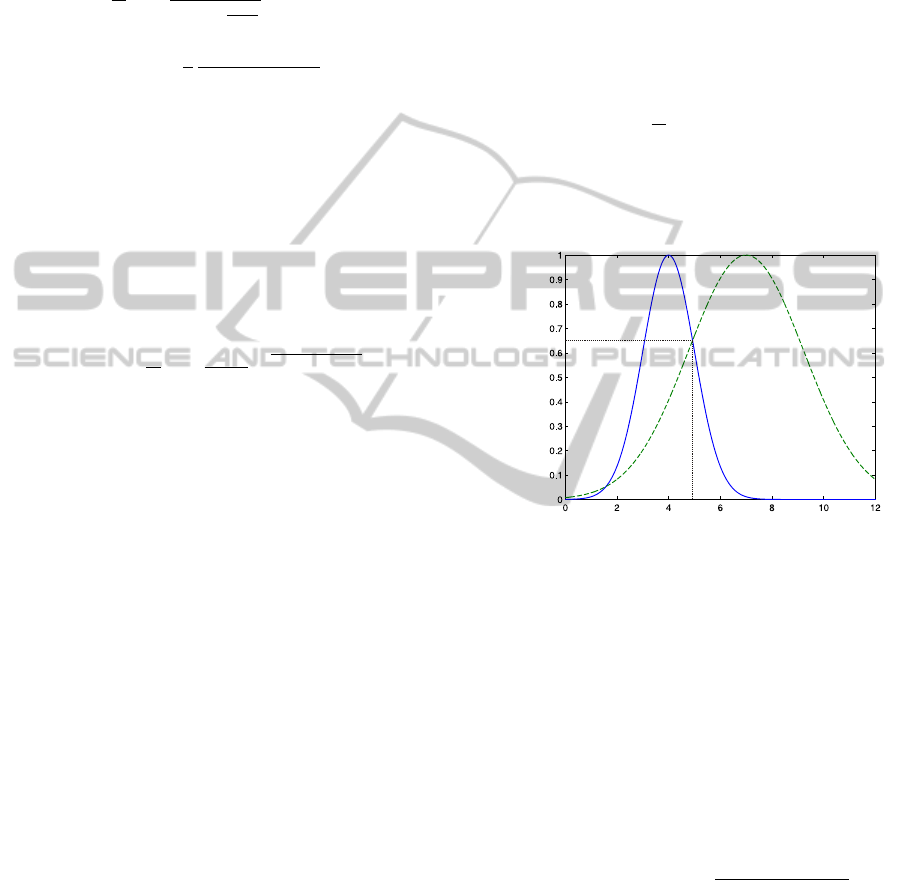
Figure 2: Example of an Assessment of the Distinguisha-
bility of two Gaussians.
Third, to simplify the understanding of a rule set,
two different rules should be easy to distinguish. This
distinguishability is only determined for the continu-
ous dimensions d ∈ {1,...,D
cont
}. It is measured by
the ordinate value of the intersection point of two uni-
variate Gaussians ϕ
d, j
and ϕ
d, j
0
(the y-coordinate of
that intersection point which has an x-coordinate be-
tween the two means, to be precise), cf. Fig. 2. This
measure is restricted to the unit interval by omitting
the normalization coefficients of the Gaussians in the
calculation which results in:
dist(ϕ
d, j
,ϕ
d,, j
0
) = 1 − exp
−
(µ
d, j
− µ
d, j
0
)
2
2 · (σ
d, j
+ σ
d, j
0
)
2
!
(24)
with dist(ϕ
d, j
,ϕ
d, j
0
) ∈ (0, 1]. Values higher than 0.3,
for example, could be regarded as desirable.
The distinguishability of the whole rule set is
given by the pair of rules which is most difficult to
distinguish, i.e., the pair with the highest value of
dist(p(x| j), p(x| j
0
)).
IN YOUR INTEREST - Objective Interestingness Measures for a Generative Classifier
419

4 CASE STUDIES
In this section we demonstrate the application of our
proposed interestingness measures by means of three
publicly available data sets. The first case study
serves as an illustrative example of the general usage
and characteristics of the measures. Then, we investi-
gates how restricting the classifier in order to produce
human-comprehensible rules influences the classifi-
cation performance. Finally, we show how some of
the interestingness measures can be used to automati-
cally prune classifiers.
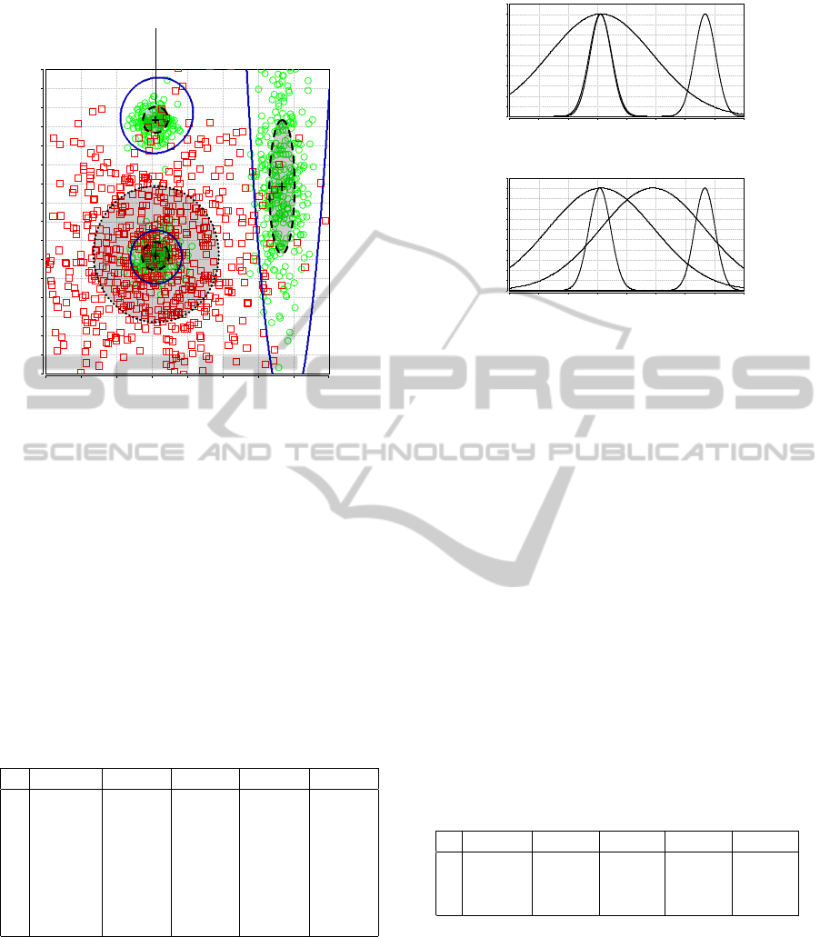
4.1 “Clouds” Data Set
The first case study uses the “clouds” data set from the
UCL/MLG Elena database (UCL, 2007). This two-
dimensional (both attributes are continuous) data set
contains 5 000 samples belonging to two classes. Fig.
3 shows a part of the clouds samples together with
a classifier trained on that data. There, the crosses
(+) describe the centers of the Gaussian components
of the trained GMM, the ellipses are corresponding
level curves (surfaces of constant density with a Ma-
halanobis distance of one to the corresponding cen-
ter) with shapes defined by their respective covariance
matrices. The solid blue line illustrates the decision
boundary of the classifier. The VI algorithm was ini-
tialized with 15 components and it pruned the final
GMM down to four. The model was trained with 75%
of the data set (i.e., 3 750 samples with a final train-
ing error of 10.6%) and tested on the remaining 1 250
samples resulting in a classification error of 9.9%.
Now, we assess this classifier by means of our pro-
posed interestingness measures. Table 1 shows the
evaluation of the four components (i.e., rules) with re-
gard to uniqueness, informativeness, importance, dis-
crimination, and representativity. First, it can be seen
that the components 1 and 3 are distant to the re-
maining two components and, thus, their informative-
ness values are quite high. Additionally, they are only
slightly covered with samples of a different class (i.e.,
the red boxes) which leads to high uniqueness values.
Components 2 and 4, in contrast, belong to different
classes and overlap. Thus, their uniqueness and in-
formativeness values are lower. Note that they exhibit
identical informativeness because they are mutually
closest to each other and the informativeness measure
is symmetric. As the class of the red boxes is only
modeled by component 4, its influence on the deci-
sion boundary (i.e., its discrimination) is high. The
class of the green circles is modeled by the remaining
three components which results in lower discrimina-
tion values that scale with their importance (i.e., the
fraction of samples they cover). Representativity is
also highly correlated with importance as the more
samples are covered by a component the higher its in-
fluence on the “goodness-of-fit”.
Table 1: Evaluation of the Component-Based Measures for
the “Clouds” Data Set.
j uniq( j) info( j) imp( j) disc( j) repr( j)
1 0.903 0.889 0.498 0.460 0.141
2 0.657 0.771 0.246 0.133 0.048
3 0.908 0.922 0.256 0.210 0.085
4 0.853 0.771 0.667 0.803 0.234
Regarding the comprehensibility of the trained
classifier it can be stated that the number of four com-
ponents is certainly very low which is a good basis for
a comprehensible classifier. Counting the number of
different univariate Gaussians in every dimension re-
quires to determine the projections of the components
onto the axes corresponding to the different input di-
mensions. The unnormalized projections of the four
components on the x- and y-axes are shown in Fig. 4.
The projections on the x-axis, Fig. 4(a), show two
nearly identical univariate Gaussians centered at -0.5
whose Hellinger distance is below 0.01. Thus, they
are regarded as being identical from the viewpoint of
comprehensibility which results in 3 univariate Gaus-
sians in the x-dimension and 4 univariate Gaussians in
the y-dimension. An average of 3.5 rules per dimen-
sion is a very good value for a comprehensible classi-
fier. The minimum distinguishability of 0.0, however,
deteriorates the comprehensibility. An example for
two components with this low distinguishability can
be seen for the y-axis projection, cf. Fig. 4(b), at the
intersection point (-0.5, 1).
4.2 “Iris” Data Set
The aim of the second case study is to investigate the
impact on classification performance when the clas-
sifier is restricted to generate human-comprehensible
rules. For that purpose, we use the well-known “iris”
data set from the UCI machine learning repository
(Frank and Asuncion, 2010). This data set contains
three classes, each with 50 four-dimensional (all con-
tinuous) samples.
First, we train a classifier without any restrictions,
i.e., with full covariance matrices. We run the VI al-
gorithm on the data set in a 4-fold cross-validation
(stratified data). With this parametrization, the result-
ing models consist of seven to ten components, de-
pending on the random initialization. The mean clas-
sification error on test data is 1.9% (std. dev. 1.1%).
Now, we evaluate the model of the last fold consisting
ICAART 2011 - 3rd International Conference on Agents and Artificial Intelligence
420
-2,0 -1,5 -1,0 -0,5 0,0 0,5 1,0 1,5 2,0
-2,00
-1,75
-1,50
-1,25
-1,00
-0,75
-0,50
-0,25
0,00
0,25
0,50
0,75
1,00
1,25
1,50
1,75
2,00
Component 1
Component 2
Component 3
?
Component 4
B
B
B
B
B
B
B
B
BN
Figure 3: CMM for the “Clouds” Data Set.
of seven components with our interestingness mea-
sures, cf. Tab. 2. The uniqueness and informativeness
measures show that all components are very “tight”
around their underlying samples and all components
are very well localized (i.e., almost no overlap). The
importance measure clearly shows four components
that cover a large portion of samples. Interestingly,
one of them has almost no impact on the decision
boundary, as shown by the discrimination measure.
As we have already stated in the first case study, rep-
resentativity is highly correlated with importance.
Table 2: Evaluation of the Component-Based Measures for
the Classifier with Seven Components and Full Covariance
Matrices.
j uniq( j) info( j) imp( j) disc( j) repr( j)
0 1.000 1.000 0.611 1.000 0.180
1 0.944 0.913 0.544 0.359 0.052
2 1.000 0.936 0.404 0.026 0.027
3 1.000 0.994 0.062 0.000 0.005
4 0.931 0.913 0.537 0.282 0.027
5 1.000 0.981 0.254 0.000 0.017
6 1.000 0.937 0.126 0.026 0.007
Regarding the classification performance it can be
seen that the VI algorithm is able to generate very
good classifiers for this data set. However, from the
viewpoint of a data miner who wants to extract inter-
esting rules, our evaluation reveals that the classifier
is too detailed and even models regions in the input
space that contain very little information.
Thus, we parametrize the VI algorithm to seek a
solution with a lower number of components which
-2,0 -1,5 -1,0 -0,5 0,0 0,5 1,0 1,5 2,0
0,0
0,1
0,2
0,3
0,4
0,5
0,6
0,7
0,8
0,9
1,0
1,1
(a) x-Axis
-2,0 -1,5 -1,0 -0,5 0,0 0,5 1,0 1,5 2,0
0,0
0,1
0,2
0,3
0,4
0,5
0,6
0,7
0,8
0,9
1,0
1,1
(b) y-Axis
Figure 4: Projection of the Gaussians onto the x- and y-Axes
for the “Clouds” Data Set.
usually results in a less detailed model. Again, we
perform a 4-fold cross-valiation which results in a
mean test error of 3.8% (std. dev. 3.8%). This time,
all four generated classifiers consist of three compo-
nents (one for each class). The results of our interest-
ingness measures for the classifier of the last fold are
listed in Tab. 3. Uniqueness and informativenes show
that one class is well separated from the remaining
two classes. The last two classes (and the respective
components) overlap to a certain degree. As every
class in this coarse-grained model is modeled with a
single component, importance shows identical values
for all components. The overlap of the classes is also
reflected by discrimination and representativity since
the well-separated component has a larger value than
the remaining two components.
Table 3: Evaluation of the Component-Based Measures for
the Classifier with Three Components and Full Covariance
Matrices.
j uniq( j) info( j) imp( j) disc( j) repr( j)
0 1.000 0.993 0.500 1.000 0.027
1 0.829 0.677 0.500 0.795 0.014
2 0.856 0.677 0.500 0.795 0.007
This result is a very good starting point to find a
comprehensible classifier. Now, we restrict the VI
algorithm to diagonal covariance matrices to enable
the extraction of human-comprehensible classifica-
tion rules. In a 4-fold cross-validation all models con-
sist of three components again and yield a mean test
error of 4.5% (Std. dev. 3.3%). Tab. 4 shows the as-
sessment of the classifier of the last fold. Compared
to the classifier with full covariance matrices unique-
ness and informativeness show similar values. Obvi-
IN YOUR INTEREST - Objective Interestingness Measures for a Generative Classifier
421

3.5 4.0 4.5 5.0 5.5 6.0 6.5 7.0 7.5 8.0 8.5 9.0 9.5
0.0
0.1
0.2
0.3
0.4
0.5
0.6
0.7
0.8
0.9
1.0
(a) 1st Dimension
1.5 2.0 2.5 3.0 3.5 4.0 4.5 5.0
0.0
0.1
0.2
0.3
0.4
0.5
0.6
0.7
0.8
0.9
1.0
(b) 2nd Dimension
0 1 2 3 4 5 6 7 8
0.0
0.1
0.2
0.3
0.4
0.5
0.6
0.7
0.8
0.9
1.0
(c) 3rd Dimension
-1.0 -0.5 0.0 0.5 1.0 1.5 2.0 2.5 3.0 3.5
0.0
0.1
0.2
0.3
0.4
0.5
0.6
0.7
0.8
0.9
1.0
(d) 4th Dimension
Figure 5: Projections of the Classifier with Three Components and Diagonal Covariance Matrices onto the Four Axes.
ously, the limited modeling capability of the classifier
due to the restricted covariance matrices has no severe
impact for this data set.
Table 4: Evaluation of the Component-Based Measures for
the Classifier with Three Components and Diagonal Covari-
ance Matrices.
j uniq( j) info( j) imp( j) disc( j) repr( j)
0 1.000 0.995 0.500 1.000 0.028
1 0.815 0.739 0.500 0.718 0.014
2 0.857 0.739 0.500 0.718 0.005
Fig. 5 illustrates the projections of the three com-
ponents onto the four axes of the input space. From
the viewpoint of comprehensibility we can state that
the number of three components (i.e., three rules) is
certainly very good. The average number of terms per
dimension is also three since there are no two Gaus-
sians that should be regarded as being identical. How-
ever, the distinguishability is very low (i.e., 0.01193).
This is due to the projections of the second dimension,
cf. Fig. 5(b), where two of the three univariate Gaus-
sians are very close to each other and, thus, difficult
to distinguish.
This case study showed that human-
comprehensible rules can be generated from a
classifier if the VI algorithm is parametrized accord-
ingly. This comprehensibility, however, comes at the
cost of a reduced classification performance as the
modeling capability of the classifier is restricted. A
compromise between understandability and classifi-
cation performance is to only reduce the number of
components while still allowing full covariance ma-
trices. Then, our proposed interestingness measures
enable a higher-level analysis of the structure of the
data.
4.3 “Heart” Data Set
Some of the proposed interestingness measures can
be used to automatically prune components from
a trained classifier. We demonstrate this with the
“heart” data set from the UCI machine learning
repository (Frank and Asuncion, 2010). This 12-
dimensional data set (six continuous and six categor-
ical dimensions) consists of 270 samples which are
partitioned into two classes. A 4-fold cross-validation
of the VI algorithm results in a mean test error of
29.13%.
We select the model from the last fold which
consists of 20 components and yields a test error of
25.0%. Then, we reduce the size of this classifier by
pruning all components whose discrimination mea-
sure is below 0.1. The mixture coefficients of the
remaining components are renormalized. The result-
ing classifier consists of only two components (which
corresponds to a size reduction of 90%) and still
achieves the same test error of 25.0% (i.e., all pruned
components had a discrimination value of 0.0).
While the reduction of the original model is cer-
tainly optimal from the viewpoint of classification
performance, it does not model the structure of the
data anymore and, thus, is not suitable for data anal-
ysis. Therefore, we used again the classifier from the
last fold with 20 components as a starting point and
pruned all components with a discrimination below
0.1 and an importance below 0.1 (i.e., components
that only cover a few data points are deleted). The
resulting model has seven components and still yields
a test error of 25.0%. This is optimal regarding the
classification performance and the interesting regions
in the input space are modeled.
Tab. 5 summarizes the results of this case study.
Certainly, it is possible to use even more interest-
ingness measures for a more sophisticated classifier
pruning. Depending on the kind of rules the data
miner is interested in, informativeness (rules that are
distant to the remaining rules, cf. exception min-
ing) or uniqueness (rules representing unambiguous
knowledge) can be used additionally.
Table 5: Pruning results.
Pruning Size Test error
none (original model) 20 25.0%
disc ≤ 0.1 2 25.0%
disc ≤ 0.1 and impo ≤ 0.1 7 25.0%
ICAART 2011 - 3rd International Conference on Agents and Artificial Intelligence
422

5 CONCLUSIONS
AND OUTLOOK
In this article, we first presented a probabilistic clas-
sifier based on mixture models (CMM) that can be
used in the field of data mining to extract classifica-
tion rules from labeled sample data. Then, we defined
some objective interestingness measures that are tai-
lored to measure various aspects of the rules of which
this classifier consists. These measures are also based
on probabilistic methods. A data miner may use these
measures to investigate the knowledge extracted from
sample data in more detail. In three case studies using
well-known data sets we demonstrated the application
of our approach.
In our future work we will investigate the pos-
sibility to apply our objective measures to each of
the C class-specific mixture models to obtain an even
more detailed class-specific assessment of the compo-
nents. In this work we used the measures as a post-
processing step to prune a trained model. However,
it is also possible to use them as side conditions in
the objective functions that are used for the training
of CMM in order to support certain properties of a
classifier already during training. Additionally, we
will investigate how the measures can be combined
to perform a ranking of rules based on their interest-
ingness. There is a close relation of CMM to certain
kinds of fuzzy classifiers concerning the functional
form as outlined in (Fisch et al., 2010). Thus, it would
also be interesting to transfer the proposed measures
to that kind of classifiers and compare them to other
measures.
REFERENCES
Atzmueller, M., Baumeister, J., and Puppe, F. (2004).
Rough-fuzzy MLP: modular evolution, rule genera-
tion, and evaluation. In 15th International Conference
of Declarative Programming and Knowledge Man-
agement (INAP-2004), pages 203–213, Potsdam, Ger-
many.
Basu, S., Mooney, R. J., Pasupuleti, K. V., and Ghosh, J.
(2001). Evaluating the novelty of text-mined rules us-
ing lexical knowledge. In Proceedings of the seventh
ACM SIGKDD International Conference on Knowl-
edge Discovery and Data Mining (KDD 2001), pages
233–238, San Francisco, CA.
Bishop, C. (1994). Novelty detection and neural network
validation. IEE Proceedings – Vision, Image, and Sig-
nal Processing, 141(4):217–222.
Bishop, C. M. (2006). Pattern Recognition and Machine
Learning. Springer, New York, NY.
Di Fiore, F. (2002). Visualizing interestingness. In Zanasi,
A., Brebbia, C., Ebecken, N., and Melli, P., editors,
Data Mining III. WIT Press, Southampton, U.K.
Duda, R. O., Hart, P. E., and Stork, D. G. (2001). Pattern
Classification. John Wiley & Sons, Chichester, New
York, NY.
Fayyad, U. M., Piatetsky-Shapiro, G., and Smyth, P. (1996).
Knowledge discovery and data mining: Towards a
unifying framework. In Proceedings of the Second In-
ternational Conference on Knowledge Discovery and
Data Mining (KDD 1996), pages 82–88, Portland,
OR.
Fisch, D., K
¨
uhbeck, B., Ovaska, S. J., and Sick, B. (2010).
So near and yet so far: New insight into properties of
some well-known classifier paradigms. Information
Sciences, 180:3381–3401.
Fisch, D. and Sick, B. (2009). Training of radial ba-
sis function classifiers with resilient propagation and
variational Bayesian inference. In Proceedings of the
International Joint Conference on Neural Networks
(IJCNN ’09), pages 838–847, Atlanta, GA.
Frank, A. and Asuncion, A. (2010). UCI machine learning
repository.
Hebert, C. and Cremilleux, B. (2007). A unified view of
objective interestingness measures. In Perner, P., ed-
itor, Machine Learning and Data Mining in Pattern
Recognition, number 4571 in LNAI, pages 533–547.
Springer, Berlin, Heidelberg, Germany.
Hilderman, R. J. and Hamilton, H. J. (2001). Knowledge
Discovery and Measures of Interest. Kluwer Aca-
demic Publishers, Norwell, MA.
Liu, B., Hsu, W., Chen, S., and Ma, Y. (2000). Analyz-
ing the subjective interestingness of association rules.
IEEE Intelligent Systems, 15(5):47–55.
McGarry, K. (2005). A survey of interestingness measures
for knowledge discovery. The Knowledge Engineer-
ing Review, 20(1):39–61.
Nauck, D. D. (2003). Measuring interpretability in rule-
based classification systems. In Proceedings of the
12th IEEE International Conference on Fuzzy Sys-
tems (FUZZ-IEEE’03), volume 1, pages 196–201, St.
Louis, MO.
Padmanabhan, B. and Tuzhilin, A. (1999). Unexpectedness
as a measure of interestingness in knowledge discov-
ery. Decision Support Systems, 27(3):303–318.
Piatetsky-Shapiro, G. and Matheus, C. (1994). The inter-
estingness of deviations. In Proceedings of the AAAI-
94 Workshop on Knowledge Discovery in Databases
(KDD 1994), pages 25–36, Seattle, WA.
Silberschatz, A. and Tuzhilin, A. (1996). What makes
patterns interesting in knowledge discovery systems.
IEEE Transactions on Knowledge And Data Engi-
neering, 8:970–974.
Taha, I. and Ghosh, J. (1997). Evaluation and ordering of
rules extracted from feedforward networks. In Inter-
national Conference on Neural Networks, volume 1,
pages 408–413, Houston, TX.
Tan, P.-N., Kumar, V., and Srivastava, J. (2004). Selecting
the right objective measure for association analysis.
Information Systems, 29(4):293–313.
UCL (2007). Elena Database. http://www.ucl.ac.be/mlg/
index.php?page=Elena.
IN YOUR INTEREST - Objective Interestingness Measures for a Generative Classifier
423
