TWO-MODES CYCLIC BIOSIGNAL CLUSTERING BASED

ON TIME SERIES ANALYSIS

Neuza Nunes, Tiago Araújo

Physics Department, FCT-UNL, Lisbon, Portugal

Hugo Gamboa

Physics Department, FCT-UNL, Lisbon, Portugal

PLUX – Wireless Biosignals, Lisbon, Portugal

Keywords: Biosignals, waves, Unsupervised learning, Clustering, Data mining, Signal-processing.

Abstract: In this paper we introduce an unsupervised learning algorithm which distinguishes two different modes in a

cyclic signal. We also present the concept of “mean wave” which averages all signal waves aligned in a

notable point (n

zero derivative). With that information the signal’s morphology is captured. The clustering

mechanism is based on the information collected with the mean wave approach using a k-means algorithm.

The algorithm produced is signal-independent, and therefore can be applied to any type of signal providing

it is a cyclic signal that has no major changes in the fundamental frequency. To test the effectiveness of the

proposed method, we acquired several biosignals (accelerometry, electromyography and blood volume

pressure signals) in the context tasks performed by the subjects with two distinct modes in each. The

algorithm successfully separates the two modes with 99.2% of efficiency. The fact that this approach

doesn’t require any prior information and the preliminary good classification performance makes this

algorithm a powerful tool for biosignals analysis and classification.

1 INTRODUCTION

Human-activity tracking techniques focus on direct

observation of people and their behavior. This could

be done, as an example, with cameras (Jezekiel Ben-

Arie, 2002), accelerometers to track human motion

(Jonghun Baek et al., 2004), or contact switches to

compute facial expressions with the

electromyography patterns (Joshua R. Smith, 2005)

(Alan J. Fridlund, 2007).

In this work we acquired several cyclic

biosignals – such as accelerometry (ACC),

electromyography (EMG) and blood volume

pressure (BVP) signals – from subjects performing

some context tasks, and we’ve developed

an unsupervised learning algorithm which is capable

to distinguish two different modes in the same

acquired signal.

The developed algorithm follows an

unsupervised learning approach, as it doesn't require

any prior information (Zoubin Ghahramani, 2004).

We use the k-means cluster algorithm due to its

efficiency and effectiveness (Xindong Wu, 2007).

As a clustering method, our algorithm is signal-

independent and doesn’t use specific information

about the signals. Although our algorithm is signal-

independent, the signals used must be cyclic signals,

with only two distinctive modes and a small

variation of fundamental frequency between those

modes.

Warren Liao (2005) presents a survey on time

series data clustering, exposing past researches on

the subject. He organizes the works in three groups:

whether they work directly with the raw data,

indirectly with features extracted or indirectly with

models built from the raw data. We created a

different algorithm as we intended to work with

single signals with different modes or activities in it,

and the previous studies uses various signals each

one distinct with only one mode or activity.

A more resemble approach, as the clustering is

based on the similarity of wave shapes presented in a

single time series data, is the work of Dr. Rodrigo

Quiroga (2007) with spike sorting. However, as the

257

Nunes N., Araújo T. and Gamboa H..

TWO-MODES CYCLIC BIOSIGNAL CLUSTERING BASED ON TIME SERIES ANALYSIS .

DOI: 10.5220/0003165002570264

In Proceedings of the International Conference on Bio-inspired Systems and Signal Processing (BIOSIGNALS-2011), pages 257-264

ISBN: 978-989-8425-35-5

 2011 SCITEPRESS (Science and Technology Publications, Lda.)

neuron activity is not periodic, the spikes are

detected with a threshold and the clustering

procedure uses features extracted from those parts of

the signal.

We present the concept of “mean wave” which

averages all signal waves aligned in a notable point,

that we call triggering point, such as maximum,

minimum, zero or inflexion point. Our algorithm

automatically separates each signal’s cycle and

computes the mean wave using an alignment on the

triggering point of each cycle. With that information

the signal’s morphology is captured. Our clustering

algorithm uses the signal’s cycles information

gathered from the mean wave approach to separates

the two modes cycles of the entire signal.

As our mean wave approach effectively captures the

morphology of a signal, can be useful in several

areas – as a clustering basis or just for a simple

signal analysis.

In the following section the signal acquisition

methodology is presented. In section 3 we expose

the signal processing detailing all algorithms steps.

Finally in sections 4 and 5 we detail and discuss our

results and algorithm performance, concluding the

work.

2 METHODS

2.1 Acquisition System and Sensors

To acquire the biosignals necessary to this study we

used a surface electromyography (EMG) sensor,

emgPLUX, a triaxial accelerometer (ACC),

xyzPLUX, and a finger blood volume pressure

(BVP) sensor, bvpPLUX (bioPLUX Research

Manual, 2010).

For the signal’s analog to digital conversion and

bluetooth transmission to the computer we used a

wireless signal acquisition system, bioPLUX

research, which has 12 bit ADC and a sampling

frequency of 1000 Hz (bioPLUX Research Manual,

2010). In the acquisitions with accelerometers just

the axis with inferior-superior direction was

connected to the bioPLUX.

2.2 Data Acquisition and Data Format

Several tasks were designed and executed in order to

acquire signals that had two distinctive modes.

We conceived a synthetic digital signal and

collected signals from four different activities

scenarios with the accelerometer sensor, and one for

each EMG and BVP sensors.

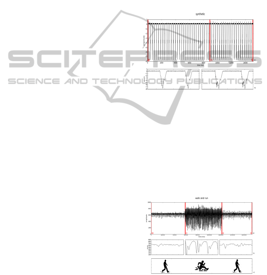
2.2.1 Synthetic Signal

To test our algorithm, a synthetic wave (Figure 1)

created using a low-pass filtered random walk (of

100 samples), with a moving average smoothing

window of 10% of signal’s length, and multiplied by

a hanning window, was repeated 30 times, so all the

cycles were identical. After a small break on the

signal the wave was repeated 20 more times, with an

identical small change of 40 samples in all waves,

creating a second mode.

Figure 1 a): Synthetic signal with identical waves from t0

to t1 and from t1 to t2; b): corresponding zoomed waves.

2.2.2 Walking and Running (ACC)

With an accelerometer located at the right hip and

oriented so the y axis of the accelerometer (the only

connected to the bioPLUX) was pointing upward,

the subjects performed a task of walking and

running non-stop (on a large circle drawn on the

floor).

The subjects walked for about 1 minute at a slow

speed, then spent 1 minute running, and ended with

1 minute walking again. The signal acquired is

represented in figure 2.

Figure 2 a): Acceleration signal of walking (t0 to t1 and t2

to t3) and running (t1 to t2); b): corresponding zoomed

waves; c): tasks performed.

BIOSIGNALS 2011 - International Conference on Bio-inspired Systems and Signal Processing

258

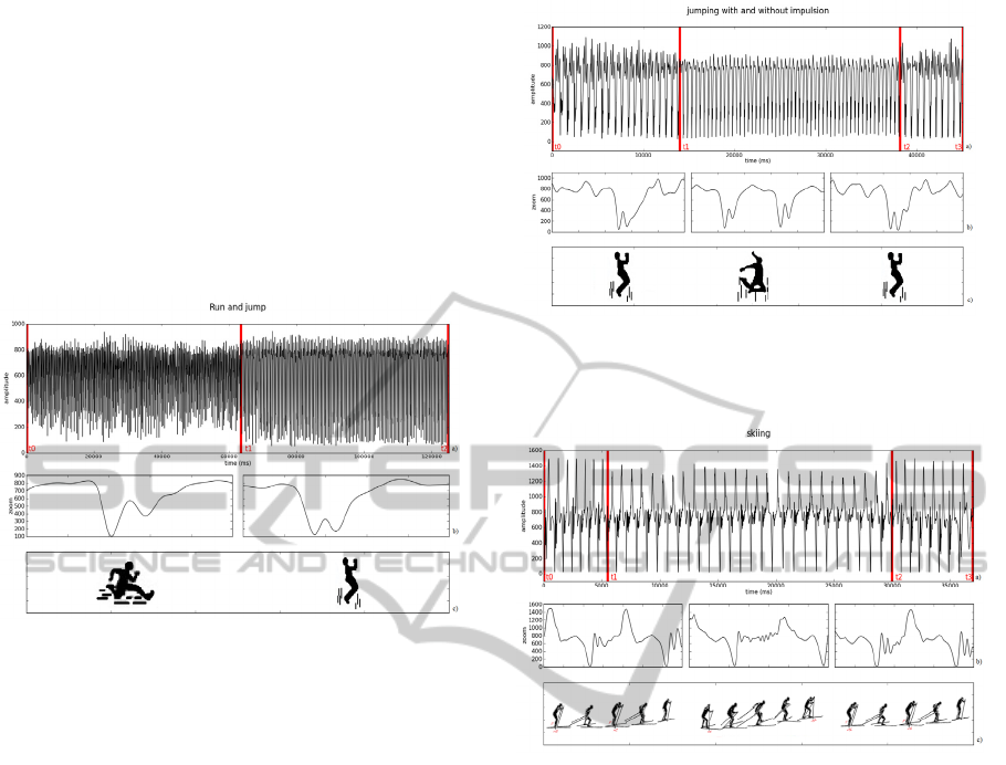
2.2.3 Running and Jumping (ACC)

With an accelerometer located at the right hip and

oriented so the y axis of the accelerometer (the only

connected to the bioPLUX) was pointing upward,

the subjects performed a task of running non-stop

(on a large circle drawn on the floor) and jumping

also continuously but at the same place.

The subjects spent 1 minute running, followed by

1 minute jumping. The signal acquired is

represented in figure 3.

Figure 3 a): Acceleration signal of running (t0 to t1) and

jumping (t1 to t2); b): corresponding zoomed waves; c):

tasks performed.

2.2.4 Jumping with and Without Impulsion

(ACC)

In this task, the following procedure was executed:

14 seconds of “normal” jumping (small jumps

without a big impulsion), 24 seconds of jumping

with some boost and again 7 seconds of normal

jumping.

The subjects used an accelerometer located at the

right hip and oriented so the y axis of the

accelerometer (the only connected to the bioPLUX)

was pointing upward. The signal acquired is

represented in figure 4.

2.2.5 Skiing (ACC)

Figure 5 shows the acceleration signal of an

accelerometer attached to the ski pole, below the

handgrip, used by the subject when skiing.

In the 37 seconds of the signal the subject

performed two different techniques, called V1 and

V2. V1 skate is an asymmetrical uphill technique

involving one poling action over every second leg

stroke. V2 skate is used for moderate uphill slopes

and on level terrain, involving one poling action for

each leg stroke. (Erik Andersson, 2010)

Figure 4 a): Acceleration signal of normal jumps (t0 to t1

and t2 to t3) and jumps with boost (t1 to t2); b):

corresponding zoomed waves; c): tasks performed.

Figure 5 a): Acceleration signal of skiing with V2

technique (t0 to t1 and t2 to t3) and skiing with V1

technique (t1 to t2); b): corresponding zoomed waves; c):

tasks performed.

The first 7 cycles of the signal (about 5 seconds)

were produced through a V2 technique, the next 27

cycles (about 25 seconds) a V1 technique and the

final 8 cycles the technique was V2 again.

2.2.6 Elevation and Squat of the Legs

(EMG)

The subject was standing straight with both feet

completely on the ground and was asked to

performed 12 elevations of the legs - getting on the

tiptoes and back with both feet completely on the

ground - followed by 11 squats - bending the knees

and back standing straight - (Figure 6). The EMG

data were collected using bipolar electrodes at the

gastrocnemius muscles of the right leg.

TWO-MODES CYCLIC BIOSIGNAL CLUSTERING BASED ON TIME SERIES ANALYSIS

259

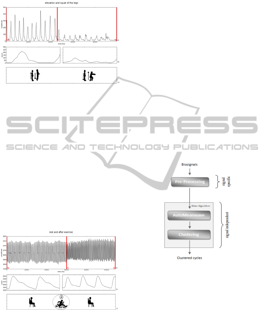
Figure 6 a): EMG signal of the gastrocnemius muscle’s

contraction through the elevation (t0 to t1) and squat (t1 to

t2) of the inferior members; b): corresponding zoomed

waves; c): tasks performed.

2.2.7 Normal (at rest) and High Beat (after

Exercise) Signal (BVP)

The subjects were instrumented with a BVP sensor

on the fourth finger of the left hand and were seating

with his left forearm resting on a platform.

We’ve made one acquisition with the subject at

rest. The subjects performed intensive exercise that

was not collected to avoid undesirable artefacts due

to movement. After the exercise, we acquired

another BVP signal.

For the purpose of this study we used both

signals (at rest and after exercise) in the same file,

cutting a part of each signal and concatenating them

offline. The resulting signal is represented in figure

Figure 7 a): BVP signal with the subject at rest (t0 to t1)

and after exercise (t1 to t2); b): corresponding zoomed

waves; c): tasks performed.

All the signals referenced above are available at

OpenSignals (Opensignals.net website, 2010).

3 SIGNAL PROCESSING

The collected data was processed offline using

Python with the numpy (T. Oliphant, 2006) and

scipy (T. Oliphant, 2007) packages.

Signal processing algorithms were developed for

automatic detection of a mean wave representative

of the signal’s behavior and the k-means algorithm

was used to cluster the signals. The main idea of this

algorithm is to define a loop with k centroids far

away from each other, take each point belonging to a

given data set and associate it to the nearest centroid.

Repeating the loop, the centroids position will

change because they are re-calculated as barycenters

of the clusters result, and after several iterations the

position will stabilize and we achieved the final

clusters (Dênis Martins, 2008).

Figure 8 describes the method used to process

the signals. All biosignals were submitted to a

signal-specific pre-processing phase and then to a

generic signal-independent phase (composed with a

mean wave and clustering procedure) which was

applied to all the signals of this study.

Figure 8: Signal’s processing procedure schematics.

For the pre-processing phase, the acceleration

signals were low-pass filtered using a smoothing

filter with a moving average window of 50 points.

The BVP signal was also low-passed filtered with

the same moving average window as the

acceleration signals. Random noise with 1/5 of

original amplitude was added to the synthetic signal.

The EMG signal was centered at y axis zero, by

subtracting its mean value, and then rectified. Then

we applied the smoothing filter with a moving

average window of 300 points.

BIOSIGNALS 2011 - International Conference on Bio-inspired Systems and Signal Processing

260

In the next sections the generic processing

procedure will be described.

3.1 Mean wave

The autoMeanwave algorithm is the base function

to identify the individual waves. After running this

algorithm we will have the mean wave computed

with the individual wave’s information.

This algorithm receives, by input, a signal, its

sampling frequency and a trigger mode (this one can

be omitted and the algorithm will use the maximum

point as default).

As we’re working with cyclic signals, the first

step of the automatic mean wave algorithm is the

detection of the signal’s fundamental frequency. For

that we use the fundamentalFrequency

algorithm. With the result we compute the window

size value and randomly selected a part of the signal

with the same number of samples as the window

size. With that signal’s part and the original signal

itself we run sumvolve algorithm to get the signal

events (series of points that we consider the center of

each cycle).

After this we have all the information necessary

to compute the mean wave, which we do in the

computeMeanwave algorithm.

Algorithm 1

autoMeanwave

Input:

Signal, sampling frequency, trigger

mode.

Output:

Fundamental frequency, window size,

events.

Next we will describe minutely the sub-

algorithms referenced above.

Algorithm 2

fundamentalFrequency

Input:

Signal, sampling frequency.

Output:

Fundamental frequency.

In the fundamentalFrequency function,

we smoothed the result of the original signal’s fast

fourier transform with a moving average window of

5% of the signal’s length. We assumed the

frequency value of the first big peak located at the

smoothed FFT signal as the fundamental frequency

of the original signal.

With the fundamental frequency value we could

compute the sampling size of a signal’s cycle. We

call that value “window size”, with a 20% margin:

winsize = (f

/ f

) *1.2 (1)

Being f

the sampling frequency and f

the

fundamental frequency. We open the window 20%

to use some more samples than a cycle.

Although there are more robust methods to

determine the fundamental frequency of a signal,

this approach is adequate for our work as the

purpose was to have a close idea of the size of a

cycle. We actually use more than one exact cycle as

we use a margin of 20%, opening the window

calculated with the fundamental frequency. Notice

that further on we use a correlation function to detect

meaningful events on a cycle, so the fundamental

frequency is just used as a preliminary estimation to

support others algorithms.

Algorithm 3

sumvolve

Input:

Two signals

Output:

Distance values.

This algorithm works as a correlation function.

Sliding the smaller window part of the signal (given

by argument) through the original signal, one sample

at a time, this algorithm compares the distance of the

two windows. We used the mean square error as the

distance function:

(2)

The result of this algorithm is a signal composed

with distance values. That distance values shows the

difference between each sliding winsize cycle and

the window selected at the first place.

After, we found all the minimum peaks of the

resulted correlation signal. Those peaks will be our

events.

Algorithm 4

computeMeanwave

Input:

Signal, events, window size.

Output:

Mean wave and standard deviation

error wave.

With the events and the window size, we cut the

signal into periods that we assume as our signal

cycles:

cycle = signal[event – winsize/2 : event

+ winsize/2]

(3)

This way, based on all cycles, we could compute

the mean value to each cycle sample, and compose a

mean wave. The standard deviation error wave is

computed with the same principle, calculating the

standard deviation error instead of the mean value.

For a better visualization of the results, we computed

TWO-MODES CYCLIC BIOSIGNAL CLUSTERING BASED ON TIME SERIES ANALYSIS

261

an error area with the standard deviation error wave

obtained. For that, we added and subtracted one

standard deviation error wave to the mean wave,

getting a superior and inferior wave, to graphically

present the error area (66% of the error). This is

shown in the results section.

After the results shown above, a final adjustment

was made: the alignment of every signal’s cycles.

The position of the mean wave’s minimum point

was detected, and that become our trigger point. The

minimum position was chosen as the trigger position

- we could use the maximum (of the signal or the

derivative), or the zero crossings, for example.

With this trigger point we recalculate the peak

events, or cutting points, used in the

computeMeanwave algorithm:

events = events + trigger – winsize/2 (4)

With the events variable recalculated, we used

the computeMeanWave function again, so the

cycles were aligned and the resultant mean wave

more accurate.

3.2 Clustering

For the clustering procedure we developed a

function that receives the signal to cluster, the

window size and cutting events produced with the

autoMeanwave algorithm.

We go through all the cutting events and for each

we select a part of the signal with center at that event

and a number of samples to both sizes equal to the

window size. Then we compare that cut with each of

the others (with the center in the others cutting

events and the same window size), using the

distance wave-to-wave formula:

Algorithm 5

distanceMatrix

Input:

Signal, Cutting events, window size.

Output:

Matrix with wave-to-wave distances.

(5)

With s

and s

being the parts of the signal selected

before.

With all of the distance values for each wave, we

built a matrix of distances.

Figure 9: Matrix of distances produced for the synthetic

waves (a)) and the skiing task (b)).

Figure 9 presents two matrixes of distances,

obtained with the imshow command. Figure 9 a)

shows the matrix of the synthetic waves distances

and figure 9 b) the matrix for the skiing task

distances. As we can see, the synthetic matrix is

almost ideal, as all the waves are equal – the

distance values only are minimums or maximums. In

the skiing matrix however, the matrix assumes a

greater variation of distances, as the cycles are not

exactly the same. However, it’s visible the similarity

between the cycles of the same technique (7 cycles

V2, 27 cycles V1 and 8 cycles V2).

To cluster the signal we used the kmeans

algorithm. Those functions received the matrix

created with the distanceMatrix algorithm and

the number of clusters expected in the data, giving

the clusters and distances to the clusters as result.

4 RESULTS AND DISCUSSION

Figure 10 shows the graphics of the resulting mean

waves (line) and deviation error area (filling) after

running the algorithms referenced above. At the left

(figure 10 a.) the graphics represent the initial mean

waves created, before the clustering procedure. At

the right (figure 10 b.) we have the mean waves

representative of the signal parts that were divided

according to the resultant clustering codebook.

It’s visible that the mean waves at the left gather

information about the behavior of the signal, even if

there are some changes in shape or frequency along

the signal. After the clustering procedure there are

some predictable variations in the resultant mean

waves. We notice an overall reduction of the

deviation error after the clustering procedure and

also a reshaping of the mean wave.

After running the clustering procedure we gather

the results for each task performed. These results are

shown in table 1.

BIOSIGNALS 2011 - International Conference on Bio-inspired Systems and Signal Processing

262

Figure 10: Mean waves of all the tasks before (a)) and after (b)) the clustering procedure.

Table 1: Clustering results.

Task

Number

of Cycles

Cycles

correctly

clustered

Errors Misses

Synthetic 50 49 0 1

Walk and run 343 342 1 0

Run and jump 296 295 1 0

Jumps 85 84 1 0

Skiing 42 41 0 1

Elevation and

squat

23 23 0 0

BVP rest and

afterexercise

165 159 4 2

All 1004 991 7 5

It is important to note that some cycles weren’t

classified, and that occurred because sometimes the

borders of the signal didn’t have a full cycle - the

distanceMatrix algorithm (algorithm 5) cannot

be used to compare a short cycle with the regular

ones. Therefore, those cycles have been rejected for

lack of pattern quality, and won’t be taken into

account.

In the “walk and run” activity there were some

extra classification points. The cycles were correctly

clustered (with only 1 error encountered), but in the

“walking” mode there were some extra points

between those cycles that were also classified. The

reason is a relatively large variation in the

fundamental frequency from the walking to the

running activity - despite one activity has all cycles

well defined (by events variable described at (4)),

the other as less than one cycle per period cut

(because of that change of fundamental frequency).

This condition shows a limitation of our algorithm –

doesn’t allow big changes in the frequency domain

in the different modes presented on the signal.

The errors of classification, note that only 7

errors were encountered, and 2 of those errors were

in transition periods – where the cycle wave is still

TWO-MODES CYCLIC BIOSIGNAL CLUSTERING BASED ON TIME SERIES ANALYSIS

263

reshaping to form the other activity and the distance

value to the mean wave or to the clusters mean

values is bigger than anywhere else on the signal.

This occurred in the jumps and in the walk and run

activities.

Given the results we can affirm that our

clustering algorithm based on the mean wave

information only returned 7 errors out of 999 cycles

with pattern quality, and therefore we achieved

99.2% of efficiency.

5 CONCLUSIONS

The proposed algorithm represents an advance in the

abstract clustering area, as it has an effective

detection of signal variations, tracing different

patterns for distinct clusters, whether it’s an activity,

synthetic or physiological signal.

6 FUTURE WORK

In future work we intend to repeat this procedure to

a wide range of subjects performing the same task,

perform a noise immunity test and also run the

algorithm using a signal with more than two modes.

We intend to introduce an automatically

perception of the cycles which are too distance from

the cluster and assign those cycles to a new

“rejection class”. This will reduce the number of

errors due to a strange cycle, in particular the

mode’s transition cycles.

The local detection of the fundamental frequency

is also a future goal, as we intend to realize when

there’s a major variation of fundamental frequency

and make our algorithms adapt its behavior

according to that variation.

Finally, we have the intention of creating a

multimodal algorithm, which can receive more than

one signal, and process those at the same time and

with the same treatment. This could be useful if we

want to use the 3 axis of an accelerometer, or

conciliate the information of a BVP with an

electrocardiography (ECG) signal.

ACKNOWLEDGEMENTS

The authors would like to thank PLUX – Wireless

Biosignals for providing the acquisition system and

sensors necessary to this investigation. We also like

to thank NIH, the Norwegian School of Sports and

Science, Håvard Myklebust and Jostein Hallén for

acquiring and allowing us to work with the Skiing

signal used in this study. We acknowledge Rui

Martins and José Medeiros for their help and advices

on the BVP acquisition procedure.

REFERENCES

Andersson, E., Supej, M., Sandbakk, Ø., Sperlich, B.,

Stöggl, T., Holmberg, H. (2010) Analysis of sprint

cross-country skiing using a differential global

navigation satellite system. Eur J Appl Physiol. DOI

10.1007/s00421-010-1535-2

Baek, J., Lee G., Park, W., Yun, B. (2004). Accelerometer

Signal Processing for User Activity Detection,

Knowledge-Based Intelligent Information &

Engineering Systems, Vol. 3215/2004, 610-617. DOI

10.1007/978-3-540-30134-9_82

Ben-Arie, J., Wang, Z., Pandit, P., Rajaram, S. (2002).

Human Activity Recognition Using Multidimensional

Indexing. IEEE Transactions on Pattern Analysis and

Machine Intelligence, vol. 24, no. 8, 1091-1104.

Fridlund, A., Schwartz, G., Fowler, S. (2007) Pattern

Recognition of Self-Reported Emotional State from

Multiple-Site Facial EMG Activity During Affective

Imagery. Society for Psychophysiological Research.,

vol. 21, no. 6. DOI 10.1111/j.1469-

8986.1984.tb00249.x

Liao, T. Warren. (2005) Clustering of time series data – a

survey. Pattern Recognition 38 (2005) 1857 – 1874.

Martins, D., Mattos, M., Simões, P., Cechinel, C., Bettiol,

J.; Barbosa, A. (2008) Aplicação do Algoritmo K-

Means em Dados de Prevalência da Asma e Rinite em

Escolares. In: XI Congresso Brasileiro de Informática

em Saúde (CBIS'2008), 2008.

PLUX – Wireless Biosignals, bioPLUX Research Manual,

PLUX’s internal report, 2010.

Quiroga, Rodrigo Q. (2007) Spike sorting. Scholarpedia,

2(12):3583

Smith, J., Fishkin, K., Jiang, B., Mamishev, A., Philipose,

M., Rea, A., Roy, S., Sundara-Rajan, K. (2005).

RFID-Based Techniques for Human-Activity

Detection. Communications of the ACM, vol. 48, no.

9, 39-44.

T. Oliphant. Guide to Numpy. Tregol Publishing, 2006.

T. Oliphant. SciPy Tutorial. SciPy, http://www.scipy.org/

SciPy Tutorial, 2007.

Wu, X., Kumar, V., Quinlan J., Ghosh J., Yang, Q.,

Motoda, H., McLachlan, G., Ng, A., Liu, B., Yu, P.,

Zhou, Z., Steinbach, M., Hand, D., Steinberg, D.

(2007). Top 10 algorithms in data mining. Knowledge

Information Systems, 14:1–37. DOI 10.1007/s10115-

007-0114-2

www.opensignals.net, last accessed on 15/07/2010

BIOSIGNALS 2011 - International Conference on Bio-inspired Systems and Signal Processing

264