
OPTIMIZING THE ASSESSMENT OF CEREBRAL
AUTOREGULATION FROM LINEAR
AND NONLINEAR MODELS
Natalia Angarita-Jaimes and David Simpson
Institute of Sound and Vibration Research, University of Southampton, Southampton, U.K.
Keywords: Cerebral Autoregulation, Linear and Non-linear system identification, Blood flow, Blood pressure,
Physiological modeling, Volterra-Wiener models, Wiener-Laguerre models.
Abstract: Autoregulation mechanisms maintain blood flow approximately stable despite changes in arterial blood
pressure. Mathematical models that characterize this system have been used in the quantitative assessment
of function/impairment of autoregulation as well as in furthering the understanding of cerebral
hemodynamics. Using spontaneous fluctuations in arterial blood pressure (ABP) as input and cerebral blood
flow velocity (CBFV) as output, the autoregulatory mechanism has been modeled using linear and nonlinear
approaches. From these models, a small number of measures have been extracted to provide an overall
assessment of autoregulation. Previous studies have considered a single – or at most- a couple of measures,
making it difficult to compare the performance of different autoregulatory parameters (and the different
modeling approaches) under similar conditions. We therefore compare the performance of established
autoregulatory parameters in addition to novel features extracted from the models’ response to a band-pass
filtered impulse. We investigate if some of the poor performance previously reported can be overcome by a
better choice of autoregulation parameter to extract from the model. Twenty-six recordings of ABP and
CBFV from normocapnia and hypercapnia in 13 healthy adults were analyzed. In the absence of a ‘gold’
standard for the study of dynamic cerebral autoregulation, lower inter and intra subject variability of the
parameters and better separation between normo- and hyper-capnia states were considered as criteria for
identifying improved measures of autoregulation. We found that inter- and intra- subject variability in the
assessment of autoregulation can be significantly improved by a careful choice of autoregulation measure
extracted from either linear or non-linear models.
1 INTRODUCTION
The active control of the diameter of small blood
vessels in the brain, usually referred to as cerebral
autoregulation (CA), protects the brain against injury
due to insufficient or excessive blood flow resulting
from a temporary drop or surge in arterial blood
pressure (ABP). Autoregulation is of great clinical
interest as it can be impaired or lost in a number of
conditions, such as stroke and subarachnoid
haemorrhage (Panerai, 1998, Panerai, 2007). In
much of the published literature, blood flow is
recorded by the safe and non-invasive Doppler
ultrasound method in response to transient changes
in ABP. Sudden deflation of a thigh cuff, large
sinusoidal variations in lower-body negative
pressure, periodic breathing or squatting, and the
Valsalva maneuver have been used to provoke larger
changes in ABP (Panerai, 1998). However the most
desirable experimental protocol for assessing
autoregulation is to record data from patients at rest
(without performing any specific maneuvers or
requiring active collaboration), especially if they are
in intensive care. Thus, many recent studies have
focused on using only spontaneous fluctuations of
ABP. While this approach increases challenges in
terms of analyzing the recorded signals and can lead
to high intra- and inter-subject variability, its
effectiveness has been demonstrated (Panerai, 1998,
Panerai et al., 1998, Panerai, 2007, among others).
Algorithms already described in the literature for
estimating autoregulation involve system
identification (black-box modeling) to represent the
relationship between ABP and CBFV. Most of the
studies of autoregulation focus on linear methods
(Zhang et al., 1998, Birch et al., 1995, Panerai et al.,
1999, 2003, Simpson et al., 2001) with the more
recent inclusion of some nonlinear approaches
251
Angarita Jaimes N. and Simpson D..
OPTIMIZING THE ASSESSMENT OF CEREBRAL AUTOREGULATION FROM LINEAR AND NONLINEAR MODELS .
DOI: 10.5220/0003164902510256
In Proceedings of the International Conference on Bio-inspired Systems and Signal Processing (BIOSIGNALS-2011), pages 251-256
ISBN: 978-989-8425-35-5
Copyright
c
2011 SCITEPRESS (Science and Technology Publications, Lda.)
(Panerai et al., 1999, Marmarelis et al., 2002,
Panerai et al., 2004, Angarita-Jaimes et al., 2010).
Although nonlinear techniques can provide
improved model fits, their benefit in assessing
cerebral autoregulation is still unclear with few
studies having systematically compared them to
linear alternatives.
In the investigation of autoregulation from linear
models, the extraction of a small number of
parameters from the frequency-, the impulse- or
step-response of the models have been studied.
Examples of autoregulatory parameters include gain,
phase and coherence in selected frequency ranges,
(Zhang et al., 1999, Panerai et al., 1999, Birch et al.,
1995, Liu et al., 2003), selected features of the step-
response (e.g. slopes, amplitudes at selected points)
(Simpson et al., 2001, Liu et al., 2003). Alternative
methods include the autoregulatory index (ARI)
(Tiecks et al., 1995), or the correlation of the ABP
and CBFV time series (Piechnik et al., 1999). The
majority of published studies have only considered a
single -or at most- a couple of measures for the
analysis of cerebral blood flow control from
spontaneous variations (Liu et al., 2003, Panerai et
al., 2001, among others) and no single method for
assessing autoregulation has become accepted as a
gold standard..
The current paper aims to contribute to
optimizing this last, but crucial step in detecting
impairment in patients’ autoregulation from the
recorded signals. In this study, we investigate the
performance of both linear and nonlinear models,
and compare different measures extracted from the
models to assess cerebral autoregulation. In the
absence of a gold standard, the autoregulatory
parameters are evaluated on a sample of signals
recorded from healthy volunteers in whom
temporary impairment of autoregulation was
induced by hypercapnia. Based on the results, we
suggest some autoregulatory measures that are most
promising for future physiological and clinical
studies.
2 METHODS
2.1 Data Collection and Pre-processing
The study was performed on 13 healthy volunteer
subjects (age 32 ± 8.8 years) and was approved by
the local Research Ethics Committee. All recordings
were made with subjects in the supine position with
the head elevated. Middle cerebral artery velocity
was measured using a Transcanial Doppler
Ultrasound system (Scimed QVL-120) in
conjunction with a 2MHz transducer held in position
by an elastic headband. Simultaneously arterial
blood pressure (ABP) was non-invasively monitored
using a finger cuff device (Ohmeda 2300 Finapress
Bp monitor). End-tidal CO2 (EtCO2) levels were
monitored via an infra-red capnograph (Datex
Normocap 200). The experimental protocol for CO2
reactivity test was as follows: each recording began
with a period of breathing ambient air for
approximately 5 minute, followed by 2 minutes of
elevated (EtCO2 ) due to the inhalation of 5% CO2
in air.
The signals were pre-processed off-line. The
maximum velocity envelope from the spectra of the
Doppler signal was extracted by fast Fourier
transform (FFT) every 5 ms. The ABP signals were
digitized at 200 Hz. Short periods of evident artifact
as well as any spikes on the signals were removed
by linear interpolation. The ABP and CBF signals
were low pass filtered (20 Hz). The start of each
heart cycle was automatically identified from the
ABP signal, after which the average ABP and
CBFVs from the right and left MCA were calculated
for each heartbeat. This time series was then
interpolated with a third-order polynomial, and
sampled at a constant rate of 5 Hz. In order to reduce
the serial correlation between samples, the signals
were further decimated to a new sampling rate of
1Hz, following anti-alias filtering with a cut-off
frequency at 0.5 Hz. These recordings were
normalized by their mean values, and the mean
values of the resultant signals were then removed. In
that way, the relative change in each signal was
obtained, and will be denoted by %ABP and
%CBFV, respectively.
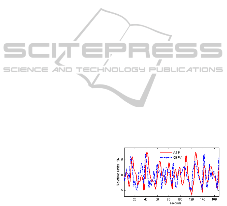
Figure 1: Representative recording, showing%ABP and
%CBFV. A phase lead of CBFV indicates a good cerebral
autoregulatory response.
2.2 Data Analysis
For each subject a segment of data was selected
from before (normocapnia – NC) and during 5%
BIOSIGNALS 2011 - International Conference on Bio-inspired Systems and Signal Processing
252
CO2 breathing (hypercapnia – HC). The former
were approx. 300 s long and the latter approx. 100 s.
For both linear and nonlinear models, %ABP
was the input and %CBFV the output. Since both
signals are normalized, the underlying assumption is
that in the absence of autoregulation changes in
%CBFV would passively follow those in %ABP
(Panerai et al., 1999). All models were estimated
according to the usual least-mean-squares approach.
A linear sixth order (5 seconds in duration) FIR filter
(Liu et al., 2005) was chosen, since the
autoregulatory response is largely completed during
this time (Panerai et al., 2003, Liu et al., 2003). A
non-linear Volterra-Wiener model, as previously
proposed (Mitsis et al., 2003, Panerai et al., 1999,
Panerai et al., 2003), was also estimated using the
Wiener-Laguerre estimation procedure (for more
details see for example Panerai et al., 1999). The
number of lags used for both the linear and nonlinear
kernels was 12.
3 ASSESMENT OF CEREBRAL
AUTOREGULATION
3.1 Selection of Autoregulatory
Parameters
A commonly used approach (Panerai et al., 1999,
Panerai et al., 2003, Liu et al., 2005) to assess
cerebral autoregulation is to look at the final value of
the models response after applying an idealized step.
From physiology, the step response is expected to
first show a sharp increase in flow when blood
pressure rises, followed by a return towards baseline
within a few seconds as autoregulation provokes
arteriolar vasoconstriction. In the absence of
autoregulation, %CBFV would remain elevated.
However, the step response shows large variability
across subjects as well as erratic variations and
decays to values less than zero that are hardly
compatible with physiology (Simpson and Birch,
2008, Liu et al., 2005) – see Fig. 2A. The relatively
narrow frequency range of spontaneous oscillations
in blood pressure is expected to lead to poor
estimation of the frequency response in the very low
and very high frequencies where the system is not
excited. This in turn probably causes the wide spread
in the final values of the step responses and the
erratic rapid variations respectively (Figure 2).
Simpson and Birch (2008) therefore proposed an
alternative test-input to assess model responses.
Instead of the step, a cosine wave modulated by a
Gaussian envelope (Fig. 2B and Fig. 3) was chosen.
This pulse reflects more closely the characteristics of
ABP from spontaneous fluctuations and its shape is
visually similar to fluctuations observed in
spontaneously varying ABP signals.
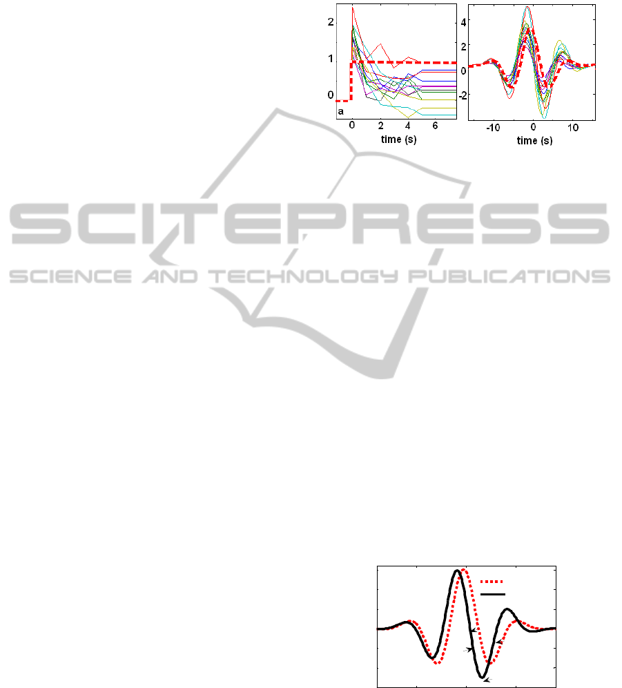
Figure 2: Step (a) and pulse (b) response for thirteen
subjects estimated from a 5 seconds-long FIR model. The
inputs are shown as the bold-dotted line. Considerably
larger dispersion is observed in the step compared to the
pulse response.
In order to quantify autoregulation using this
response, , four parameters were selected, as shown
in Fig. 3: the time of the left shift of the response
(TLS, in seconds), measured as the difference in
time between input and output crossing the abscissa
after the main peak, the amplitude of the pulse
response at 1.5 seconds (A1.5), the amplitude at 6
seconds (A6) and the time of the second negative
peak (TP) - for the input signal this occurs at 3.5
seconds. These parameters were chosen as they
reflect the expected left-shift (phase-lead) of the
autoregulatory response, and had been found most
robust in preliminary work; A1.5 and A6 lie on the
steep slopes of the descending and ascending
responses, and are therefore likely to be most
sensitive to temporal shifts in the response.
We compare these novel parameters with others
previously proposed in the literature. First, we
estimated the final value of the step response (FVS)
for both the linear and nonlinear models. Then, for
-10 0 10
-3
-2
-1
0
1
2
3
time (s)
%
Input
Output
A6
TP
TLS
A1.5
Figure 3: The %ABP test input (dotted line - sinusoid
modulated by a Gaussian pulse) and the estimated
response (solid line - %CBFV), together with the
parameters used to quantify autoregulation.
OPTIMIZING THE ASSESSMENT OF CEREBRAL AUTOREGULATION FROM LINEAR AND NONLINEAR
MODELS
253
the linear models, the average phase (Pha) was
calculated from transfer function analysis in the
frequency range from 0.07 Hz to 0.2 Hz (Zhang et
al., 1998, Birch et al., 1995), and coherence, (Coh)
was evaluated over a similar range (Zhang et al.,
1998, Panerai et al., 1998). The correlation method
(Mx) was also estimated from the average Pearson’s
correlation coefficient of 4 equal segments of the
%ABP and %CBFV time series (Piechnik et al.,
1999). The Autoregulatory Index ARI was
calculated from the set of models proposed by
Tiecks et al. (1995). For each recording, the set of
models was applied to the %ABP, and the model
leading to the highest correlation coefficient
between the model generated velocity and the
measured %CBFV gave the ARI. Finally, a
parametric model based on the coefficients of a first-
order (two taps) FIR filter was evaluated. The
second coefficient of the filter H1 was selected as it
has been shown to reflect autoregulatory activity
(Simpson et al., 2001).
3.2 Statistical Analysis
The aim of estimating autoregulatory parameters is
to be able to distinguish between impaired and
normal autoregulation. Since hypercapnia is known
to impair autoregulation, changes in the
autoregulatory parameters in response to increased
pCO
2
were tested using Wilcoxon matched pairs
tests. In addition repeatability and intra- and inter-
subject variability were also evaluated. Inter-subject
variability was assessed by calculating the standard
deviation during normo and hypercapnia, and
averaging the result (SD). In order to compare the
performance of parameters, SD was normalized by
the difference in mean value between NC and HC
(CVd).
To investigate the effect of noise and as an
indication of the repeatability of the autoregulatory
parameters, 100 simulated signals were generated
from each of the recordings. Additive noise was
modeled based on the residual error in %CBFV (i.e.
the signal component that cannot be explained by
applying the identified models to the %ABP signals)
using an AR model of order 8. Surrogate %CBFV
signal were then generated by applying the identified
models (linear or nonlinear) to the %ABP signals
and then adding the random noise to simulate
residuals. Autoregulation parameters were then
calculated from these simulated signals, and their
standard deviation was considered as the intra-
subject variability for each recording and parameter.
These were also normalized by the parameter’s
mean difference between normocapnia and
hypercapnia, and their average across the subjects
was denoted by mCVd. Low values of CVd and
mCVd indicate low dispersion and wide separation
between groups.
For each model, the predicted velocity response
was also compared to the measured data and the
model’s performance was evaluated using the
normalized mean square error (NMSE). Cross-
validation, with two equal segments, was used to
calculate NMSE.
4 RESULTS
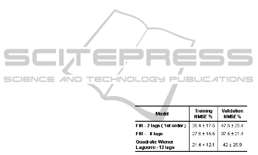
Table 1 shows the NMSE in fitting different models
to the data. The most sophisticated model has the
smallest error on the training data (150 s duration)
but on the validation data set performs poorly. The
simplest model (1
st
order FIR) overall shows the
poorest model fit, both on training and validation
data.
Table 1: Mean ± SD NMSE across 13 subjects for the
different models used on baseline recordings.
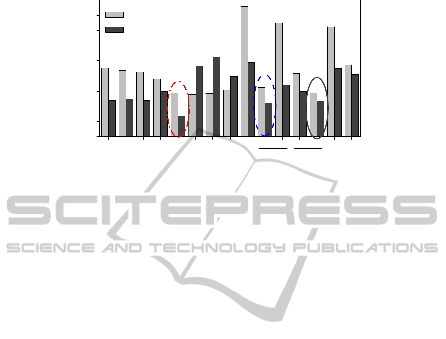
The performance of the different autoregulatory
parameters is shown in Figure 4, and provides a
rather different picture of which model might be
most appropriate in quantifying autoregulation. CVd
and mCVd estimates, indicating inter- and intra-
subject variability respectively, are presented for all
10 parameters studied. The last five were evaluated
for both the linear (L) and nonlinear models (NL).
Autoregulatory parameters with the smallest
CVd indicate best separation between NC and HC,
and can thus considered to provide the clearest
distinction between normal and impaired
autoregulation in terms of inter-subject variability.
Amongst the parameters studied H1, TP (both for
linear and nonlinear models), A1.5 (linear model)
and A6 (nonlinear model) had the lowest CVd. The
latter three show a clear improvement compared to
the final value obtained from the step response
(FVS). Furthermore, Wilcoxon matched pair test
showed that the magnitude of these parameters
BIOSIGNALS 2011 - International Conference on Bio-inspired Systems and Signal Processing
254
Mx Pha Coh ARI H1 L NL L NL L NL L NL L NL
0
20
40
60
80
100
120
140
160
180
+
o
o
o
*
*
+
*
*
*
o
o
*
FVS
A6
A1.5
TLS
TP
CVd
Inter-subject variability
mCVd
Intra-subject variability
%
Autoregulatory Parameter
Figure 4: Comparison of the different autoregulatory parameters. L (linear) and NL (non-linear) models, respectively. The
different significance levels of the Wilcoxon test comparing parameters during NC and HC are grouped as: + 0.009<p <
0.0009; * 0.09< p ≤ 0.009, o p≤0.09 (inter-subject variability) The parameters showing the strongest distinction between
NC and HC for linear and non-linear models, are circled.
changed significantly between NC and HC (H1,
p≈0.0014; TP-L, p≈0.0006; TP-NL p≈0.002, A1.5-
L p≈0.004; A6-NL p≈0.0006).
The different measures performed differently
depending on the models used to characterize the
relationship between ABP and CBFV. For example,
whilst the amplitude at 1.5 s or TLS performed well
with the L model, these had very high inter-
individual dispersion for the NL approach.
Conversely, amplitude at 6 s was the best parameter
for the NL and poorer for L. A slight improvement
in FVS was observed by using the NL approach.
When evaluating the influence of additive noise
in the recordings, the highest dispersion in terms of
mCVd (see Figure 4, darker bar) was noted for the
non-linear models, and especially the time-delay
parameters. In some cases the mCVd was larger than
CVd, which probably reflects the differences in
normalization: in the former dispersions are
normalized by the differences for each individual
(and then averaged across the cohort), but in the
latter it normalization is by the average difference.
Conventional parameters extracted from the
frequency response (Pha, Coh) as well as Mx were
relatively robust to noise (low mCVd). Overall, the
autoregulatory parameters with the lowest variability
and best separation between pC02 levels are H1,
A1.5 (linear model) and A6 (nonlinear model). The
excellent performance of the simplest parameter,
H1, is particularly notable, and is shown in more
detail in Figure 5, with 12 of 13 subjects showing
the expected increase in H1 during HC.
5 DISCUSSION
In previous work, the high inter-subject variability
of a number of measures of cerebral blood flow
control and poor repeatability has been noted
(Panerai et al., 2003, Simpson et al., 1999). The
results in this work showed that the model used to
represent the relationship between blood flow and
blood pressure, and how the models are then used
(the calculation of autoregularory parameters), can
notably increase the uncertainty in the estimates.
The current work is probably the most extensive
comparison between different parameters of
autoregulation published to date. In some of the
earlier work (Panerai et al., 1999, Panerai et al.,
2003, Mitsis et al., 2004, Angarita-Jaimes et al.,
2010) the primary concern has been with how well
different models fit the data. This however is only an
intermediate step in addressing the main challenge:
quantifying autoregulation when only spontaneous
fluctuations in ABP and CBFV are present. In the
continued absence of a gold-standard measure of
autoregulation, we take as criteria for assessing
performance the ability to distinguish between
normal (during normo-capnia) and impaired (during
hyper-capnia) autoregulation. The current work also
moves beyond the more established ‘test inputs’ that
give impulse, step or frequency (i.e. sine-wave)
responses, recommending a ‘test input’ that is
physiologically more realistic, in the form of a
broad-band pulse.
Larger dispersion was observed in the traditional
autoregulatory parameters, particularly in the final
OPTIMIZING THE ASSESSMENT OF CEREBRAL AUTOREGULATION FROM LINEAR AND NONLINEAR
MODELS
255

value of the step response, compared to some of the
measures extracted from the pulse response, as
indicated by CVd (see Figure 4). The simulations
indicate that intra-subject variability, due to assumed
additive noise in the recordings is a large contributor
the overall dispersion in results. However in this
respect, H1 outperformed all other measures. H1
was also among the best in terms of inter-subject
variability. It should also be noted that model fit
(Table 1) alone clearly is not a good indicator of
what makes for the best method in the assessment of
autoregulation.
Figure 5: a) Magnitude of H1 during normocapnia (NC)
and hypercapnia (HC). b) Box plots representation of the
median, quartile, minimum and maximum of H1.
A number of other parameters for assessing
autoregulation, including parameters taken directly
from the model (as H1 for the first order FIR filter)
were also investigated, but none proved superior to
the ones presented. The relatively small sample of
recordings available and relatively large number of
parameters tested is a limitation of the current study.
It is possible that the relative performance of the
methods reflects peculiarities or random effects in
the particular data set available. Given that
parameters estimated are not independent, the usual
methods for determining statistically significant
differences between the approaches are not
appropriate. However, the large differences observed
between methods, probably do indicate which
approaches are most promising to be taken on in a
further study on a larger data set.
6 CONCLUSIONS
In this work we have compared a number of
measures to evaluate autoregulatory activity. Some
of the parameters extracted from the proposed pulse
input show less variability compared with the more
conventional parameters extracted from the
frequency and step responses. Thus relatively small
variations across as well as within subjects were
found for the amplitude of the pulse response at
certain lags (A1.5, A6). These also showed a clearer
distinction between the different levels of
autoregulation (quantified by the p value). In
particular, for linear models A1.5 would be
recommended whereas A6 seemed to perform well
for nonlinear models. However, the results obtained
from H1 suggest that this parameter from a very
simple model might be the method of choice, with
small coefficients of variation (CVd, mCVd). This
method also allows the analysis of relatively short
data segments and thus lends itself to further studies
of time-varying (adaptive) estimates of dynamics in
cerebral blood flow control.
ACKNOWLEDGEMENTS
We would like to thank Drs. Stephanie Foster and
Lingke Fan and Prof. David Evans (Leicester Royal
Infirmary) for generously providing the anonymized
data used in this study and Innovation China UK for
funding support.
REFERENCES
Aaslid, R. et al., 1989 Cerebral autoregulation dynamics
in humans. Stroke, 20:45-52.
Angarita-Jaimes, N. et al., 2010. Nonlinear modelling of
CA using cascade models. Proc. Medicon 2010,
Greece.
Birch, A. et al., 2002. The repeatability of CA using
sinusoidal lower -ve pressure. Phys. Meas, 23,73-83
Liu, Y. et al., 2003 Dynamic cerebral autoregulation
assessed using an ARX model. Med. Eng. Phys., 25.
Liu, J. et al., 2005. High spontaneous fluctuation in ABP
improves the assessment of CA. Physiol. Meas, 26
Mitsis, G. et al., 2004 Nonlinear modelling of dynamic
CBF in healthy humans. Adv Exp Med Biol. 551:259-
265.
Panerai, R. et al., 1998. Grading of CA from spontaneous
fluctuations in ABP. Stroke, 29:2341-2346.
Panerai, R. 1998. Assessment of CA in humans -a review
of measurement methods. Physiol.Meas. 19.
Panerai, R. et al., 1999. Linear and nonlinear analysis of
human dynamic CA. Am J Heart Circ Physiol. 277
Panerai, R. et al., 2003. Variability of time-domain indices
of dynamic CA Physiol Meas, 24:367–381.
Piechnik, S. et al., 1999 The continuous assessment of
cerebrovascular reactivity Anesth Analg, 89:944–9
Simpson, D. et al., 2001. A parametric approach to
measuring CA Ann Biomed Eng, 29:18–25.
Simpson, D. and Birch, A., 2008. Optimising the
assessment of CA from black-box models. Proc.
MEDSIP 2008.
Tiecks, F. et al., 1995. Comparison of static and dynamic
CA measurements. Stroke 26: 1014-1019.
Westwick, D. and Kearney, R., 2006. Identification of
Nonlinear Physiological Systems. IEEE Press, 1st Ed.
Zhang R et al., 1998 Transfer function analysis of dynamic
CA in humans. Am. J. Physiol., 274.
BIOSIGNALS 2011 - International Conference on Bio-inspired Systems and Signal Processing
256
