
AUTOMATIC SEGMENTATION OF CONDUCTIVITY CHANGES
IN ELECTRICAL IMPEDANCE TOMOGRAPHY IMAGES
A. Zifan, P. Liatsis, P. Kantartzis and R. Vargas-Canas
School of Engineering and Mathematical Sciences, City University, London, U.K.
Keywords: Electrical impedance tomography, Mesh, Probabilistic modeling and segmentation.
Abstract: In this paper, we propose a novel method for the automatic segmentation of Electrical Impedance
Tomography (EIT) lung images. EIT is a non-invasive technique, which produces low-spatial and high-
temporal resolution images of the internal resistivity of the region of the body probed by currents. EIT is the
only technology that reliably quantifies regional lung volumes non-invasively. The problem is non-linear
and ill-conditioned and can be solved using 2D or 3D finite element methods (FEMs) subject to using
appropriate regularisation strategies. The usual method of segmenting EIT lung images is to manually select
a region of interest and derive statistical measures. This procedure is not suitable for FEM-based models as
it works on rectangular pixels, as well as making the task tedious and time consuming. We propose an
alternative segmentation framework, which operates directly on the resulting FEM meshes, prior to
rasterisation in order to prevent the propagation of errors in the reconstructed resistivity regions, due to
mapping onto a rectangular grid. We use a spatio-temporal probabilistic method to segment conductivity
changes in the EIT thorax images. Application of the proposed method offers a much needed alternative to
interactive segmentation currently favoured by EIT researchers and clinicians.
1 INTRODUCTION
EIT is a non-invasive technique, which produces
images of the internal conductivity or resistivity of
the region of the body probed by alternating currents
(Brown, 2003). EIT could be applied to imaging
both structural and functional abnormalities in the
human lungs. It has several advantages over existing
chest-imaging techniques, including low cost,
portability, its non-invasive and non-ionizing nature,
the potential for ambulatory or ICU measurements
and fast acquisition speed. EIT is the only non-
invasive technique that provides insight into the
regional distribution of ventilation. Current
strategies to provide lung protective ventilation rely
on avoiding lung over distension by reducing tidal
volumes and on opening atelectasis by applying
adequate positive end-expiratory pressure. However,
it is currently impossible to continuously measure
regional lung over distension and atelectasis while a
patient is ventilated, but it would be extremely
relevant information that could lead to reducing
ventilator-induced lung injury. EIT can resolve
changes in the distribution of lung volumes between
dependent and non-dependent lung regions as
ventilator parameters change. Thus, EIT
measurements may be used to control the specific
ventilator settings to maintain lung protective
ventilation on an individual patient basis (Frerichs et
al, 2006).
In EIT, current density flow within the body is
described by Maxwell’s equations. Typically,
multiple electrodes are placed on a person's thorax
and a sinusoidal current excitation is imposed. The
governing equation for the voltage field produced by
placing a current across a material is
()0
σ
ωε ϕ
∇
⋅+ ∇=
(1)
which is an elliptic partial differential equation,
where σ is the electric impedance of the medium, φ
is the electric potential, ω is the frequency, and ε is
the electric permittivity (Molinari, 2003). Equation
(1) is reduced to the standard governing equation for
EIT
, ()0
σ
ϕ
∇
⋅∇ = when the angular frequency is
sufficiently low or direct current is used.
By repeating these steps and scanning around
various electrode pairs, it is possible to calculate the
approximate current distribution inside the body
through inverse solution of Maxwell's equations
using two or three-dimensional finite element
215
Zifan A., Liatsis P., Kantartzis P. and Vargas-Canas R..
AUTOMATIC SEGMENTATION OF CONDUCTIVITY CHANGES IN ELECTRICAL IMPEDANCE TOMOGRAPHY IMAGES.
DOI: 10.5220/0003157002150220
In Proceedings of the International Conference on Bio-inspired Systems and Signal Processing (BIOSIGNALS-2011), pages 215-220
ISBN: 978-989-8425-35-5
Copyright
c
2011 SCITEPRESS (Science and Technology Publications, Lda.)

methods. A medical image can then be
reconstructed, since the structures within the human
body have different resistivities. However, this
requires the solution of a non-linear, ill-conditioned
inverse problem. The non-linearity arises in σ, since
the potential distribution. φ, is a function of the
impedance, φ= φ(σ), and the ill-conditioning stems
from the fact that small errors in the measurements
or in the forward modelling step may introduce large
errors in the reconstruction. The forward problem in
EIT is to estimate the induced electrical
measurements at the electrodes, given an excitation
signal and permittivity distribution. The inverse
problem estimates the permittivity distribution based
on the excitation signal and the terminal electrical
measurements. Once images have been
reconstructed, following regularization of the
inverse problem, in the final stage, FEM
triangulation results are rasterised to cover a
rectangular grid for subsequent image processing.
2 EIT LUNG IMAGES
2.1 Low Spatial Resolution of EIT
Images
It is well known that a reconstructed EIT image is
unique for noise-free complete boundary data
(Sylvester and Uhlmann, 1986). However, in
comparison to magnetic resonance imaging (MRI)
and computed tomography (CT), EIT suffers from
poor spatial resolution due to noise, low sensitivity
of boundary voltages to inner conductivity
perturbations and a limited number of boundary
voltage measurements (Clay and Ferree , 2002).
Moreover, the reconstructed images are usually
subtracted from a reference frame in order to
minimize errors due to electrode movement or
unknown boundary shape. A comparison of an EIT
image and its CT counterpart of the thorax is shown
in Figure 1. In spite of the above, EIT is very useful
in monitoring patient lung volume, because the air
has a large conductivity contrast compared to other
tissues in the thorax. The large change in lung
impedance with respiration, and the ease of use of
impedance tomography as a monitoring technique,
has led to a significant body of research in lung
impedance (Frerichs, 2000). However, the spatial
resolution of the EIT images reduces further with the
rasterisation process, where FEM model results are
mapped onto a rectangular grid for further image
processing. This rasterisation step introduces further
fuzziness to the reconstructed regions of
conductivity changes in the EIT images of the lungs,
and makes it even harder to determine the outline of
these rapidly changing regions during the breathing
cycle.
(a) (b)
Figure 1: (a) CT image of the thorax (Ackermann, 1995)
(b) EIT difference image (brighter regions correspond to
larger conductivity changes).
2.2 Feasibility of EIT Image
Segmentation
Due to the aforementioned problems regarding the
poor spatial resolution of EIT images, a question
arises as to whether it is possible to introduce a
robust adaptive EIT segmentation method.
Currently, there exists no method, which could
automatically segment regions with significant
conductivity changes, corresponding to the lobes for
an entire EIT breathing cycle sequence. The usual
method of segmenting or interrogating images is to
select a region of interest (a pixel or a small region)
on the image and then derive statistical measures for
the selected regions (Smallwood, 1999).
An additional problem is that EIT patient
histories generally include data from a limited
battery of tests, thus, making it difficult to train a
sufficiently complete probabilistic model.
Traditional background subtraction algorithms are
not appropriate due to the slower inflation/ deflation
rate of the lungs compared to the acquisition frame
rate (i.e., 13 fps), hence changes in the lung lobe
conductivity images appear slow moving or
temporarily stationary. Under these conditions, the
background becomes corrupted and object/blob
detection becomes erroneous.
To address the above issues, in the following
section a two-fold approach is proposed to tackle
this. In the first step, we carry out segmentation on
the FEM meshes prior to the rasterisation stage. This
prevents regions becoming even fuzzier and
facilitates the estimation of accurate measurement
results, which is a prerequisite for the extraction of
much needed ventilation parameters. In the second
step, we use a probabilistic model, which
accommodates both temporal and spatial contiguity
of mesh element values in order to segment and
BIOSIGNALS 2011 - International Conference on Bio-inspired Systems and Signal Processing
216

extract regions of conductivity changes directly from
the EIT lung FEM meshes.
3 METHOD
3.1 Dealing with Non-rectangular
Grids
The basis of the proposed approach is segmentation
of conductivity changes on the actual FEM meshes,
rather than the post-processed, rasterised images.
This necessitates assigning a label to each triangular
or tetrahedral element on the FEM mesh in order to
access their coordinate positions. Unlike traditional
images, which are typically based on rectangular
grids, meshes can be of any shape and their
constitutive elements maybe triangles in 2D or
tetrahedra/ hexahedra in 3D. This restricts the
applicability of image processing approaches, which
are commonly implemented on rectangular grids. In
the proposed method, we use the centroid of each
triangular element composing the mesh (in our case,
a 2D cross section of the thorax) as the
representative of that particular element and we
repeat this for all elements in the mesh. The
coordinates of the centroids form the inputs for
subsequent processing. A visual interpretation of the
centroid concept on a sample mesh of the thorax
obtained from EIDORS (Adler, 2006) is shown in
Figure 2.
The next stage of the method consists of three
steps. Firstly, we use anatomical information
regarding the position of the lungs in the thorax to
extract elements belonging to the background and
obtain a prior model of the background by fitting a
Gaussian to the trajectory of each background
element value,
Bkg
E , as it varies in time. Secondly,
the change of mesh element values through time is
modelled as an ‘element process’ and a Gaussian
probability distribution is fitted to this
trajectory,
ele
E . Thirdly, an additional model,
corresponding to the change of the sum of each
element’s neighbourhood associations through time,
is formed by fitting a Gaussian probability model.
The term ‘neighbourhood association’, denotes the
connectivity neighbourhood value
.conn
E of mesh
element
),(
θ
rE , where ),(
θ
r are the polar
coordinates of the elements’ centroid, which consists
of the number of adjacent triangles in the mesh that
share a common edge with the current element. An
example of neighbourhood association of the 251
st
element is shown in red patches in the mesh of
Figure 2.
Figure 2: Centric assigned to each mesh element.
For this particular element the connectivity
parameter will be
()
∑
=
−=
3
1
),(),(
i
iiconn
rErEE
θθ
(2)
This parameter will be calculated for all elements
in each frame in the sequence and a Gaussian model
will be fitted to its trajectory. Finally, each new
mesh element is classified by the closeness of its fit
to the three Gaussian distributions (i.e.,
Bkg
E
,
ele
E
and
.conn
E ).
3.2 Statistical Background Model
As previously discussed, the first task involves
modeling of the background. This is achieved by
using anatomical structure of the lung lobes. As
observed in Figure 1(a), several layers exist between
the lung lobes and the surface of the skin, i.e., skin
tissue, fat layers, muscles covering the thorax and
the thoracic skeleton, which protects the lungs.
(a)
(b)
Figure 3: (a) Image progression is from left to right, top to
bottom. Full-breath cycle is shown. (b) Variance mesh
(Brighter regions correspond to higher conductivity
variance).
AUTOMATIC SEGMENTATION OF CONDUCTIVITY CHANGES IN ELECTRICAL IMPEDANCE TOMOGRAPHY
IMAGES
217

This suggests that elements close to the boundary
of the thorax do not form part of the lung lobes and
thus background samples maybe extracted from
these regions. In order to validate this hypothesis,
we consider a sequence of reconstructed EIT FEM
images corresponding to one of the patients in our
dataset. The cycle is shown in Figure 3(a).
Next, we calculate the variance of each element
over this period, and produce a variance image, as
shown in Figure 3(b). As it is clearly seen, the lung
lobes display the highest conductivity changes,
followed by the adjacent darker region (depicted in
red and black colours), which separates them from
the other layers; we were able to reproduce such
variance ‘pattern’ images for all patients in the
dataset. Hence, the two most distant element layers
from the mesh centre were used as background
samples. For all of these elements in a frame
sequence, we model their change trajectory as a
random variable that follows a Gaussian
distribution
),(~
2
,,, jijiji
p
σμ
Ν
.
2
2
2
)(
,
,
2
,
1
)),(
,
(
,
ji
ji
x
e
ji
r
ji
E
ji
p
σ
μ
πσ
θ
−−
=
(3)
where
ji
p
,
is a pixel-wise random variable which
follows a Gaussian distribution, located at the
th
j
position in the
th
i EIT frame sequence. ),(
σ
μ
are
the corresponding mean and standard deviation
parameters of the Gaussian distribution. Hence,
background mesh element values over time are
modelled as a time series, which is called an element
process.
Methods employing time-adaptive per-pixel
mixture of Gaussians (MoG) are a popular choice
for modelling scene backgrounds at the pixel level
(Stauffer, 1999). In our application, one Gaussian
sufficed, and moreover such methods are not
appropriate for EIT, since we are not interested to
merely segment out the foreground, but rather the
lung lobes. This is better understood by examining
Figure 3(b). It can be clearly seen that the current
background model is not sufficient for lung lobe
conductivity change segmentation. Specifically, the
central region mesh elements also exhibit constant
changes of conductivity; however, they do not
belong to the lung lobes. For example, if we
threshold the elements of this mesh using the 75
percent Quantile of the variance values we get the
FEM shown in Figure 4.
As it can be seen in this figure, central regions
also show a large degree of change in conductivity,
Figure 4: Thresholded variance image.
hence a Gaussian model fitted to the mesh element
trajectories could indeed belong to the foreground;
however, it may not necessarily form part of the
lobes, which is the objective of this work. In order to
resolve this problem, we build two further element
process models, namely
ele
E and
.conn
E , the first
representing changes of an individual element in
time (excluding previous elements used for the
background model) and the second representing the
region attribute process in time, as discussed before.
So, if the new element centroid was not classified as
part of the initial background model, it would be part
of the foreground but it may or not correspond to the
lobe regions that we are after. Next, by comparing
its value to our other two probabilities calculated
for
ele
E and
.conn
E we can then calculate whether it
maximizes both these probabilities ensuring which
only an element in the lobe region might do.
3.3 Element Classification
Each background element has its own threshold
value, which can be obtained from the
corresponding standard deviation. In this respect, the
proposed method is similar to the adaptive method
described in (Stauffer, 1999), i.e., a per-element/per-
distribution thresholding method. The details of the
algorithm are as follows:
1) Calculate Background model
),(
bgbg
N
σμ
2) For each element in current frame calculate
}2,1{),,( =−=Η etrE
ieiie
μθ
,
3)
ieie
η
σ
=
Τ
,
bgbg
η
σ
=
Τ
4) if
bgie
T<Η
then element is background,
update background. Go to Step 6 else it’s a
possible lobe
5) if
bgie
T>
Η
&
ieie
T>
Η
element belongs
to the lung lobe region. Go to Step 2.
6) ),,()1( trE
iieie
θ
α
μ
α
μ
+
−
=
),,()1( trE
iieie
θ
α
σ
α
σ
+
−
=
Here,
),,( trE
i
θ
is an element in a current frame
(
th
i in the sequence),
1i
μ
is the mean of the
BIOSIGNALS 2011 - International Conference on Bio-inspired Systems and Signal Processing
218
element-wise Gaussian distribution,
2i
μ
is the mean
for the regional attribute distribution,
21
,
ii
σ
σ
are
the corresponding element-wise standard deviations,
respectively,
ie
Η is the absolute difference between
i
E and the distribution means,
bg
T
and
ie
T are the
element-wise thresholds for
Bkg
E ,
ele
E and
.conn
E ,
α
is the learning rate of the background and
η
is
the threshold gain.
),(
bgbg
N
σμ
is pre-calculated
and is not updated to accommodate for faster
computation speed.
4 EXPERIMENTS AND RESULTS
4.1 Data Acquisition and Processing
Data were collected from a group of 10 male
subjects with no known respiratory or cardiac
abnormalities (age: mean 32; age range, 27-42). In
each case, the 16 element adjacent electrodes were
placed around the subject’s lower thorax (4
th
-6
th
intercostal space on the mid-clavicular line). The
subjects lay supine, and were asked to relax and
breathe normally during a 3 min recording. A total
of 2340 frames were recorded using a Sheffield
mark 1 EIT system, using a 50 kHz current drive
(Brown B. H. and Seagar A. D., 1987).
The measured voltage data were then imported
into EIDORS and the inverse problem was solved
using the Gauss-Newton reconstruction algorithm on
a 2D, 576-element thorax mesh model, shown in
Figure 2. The FEM triangulation results were not
parameterized on a 2D pixel grid after the
reconstruction, in order to prevent further resolution
deterioration.
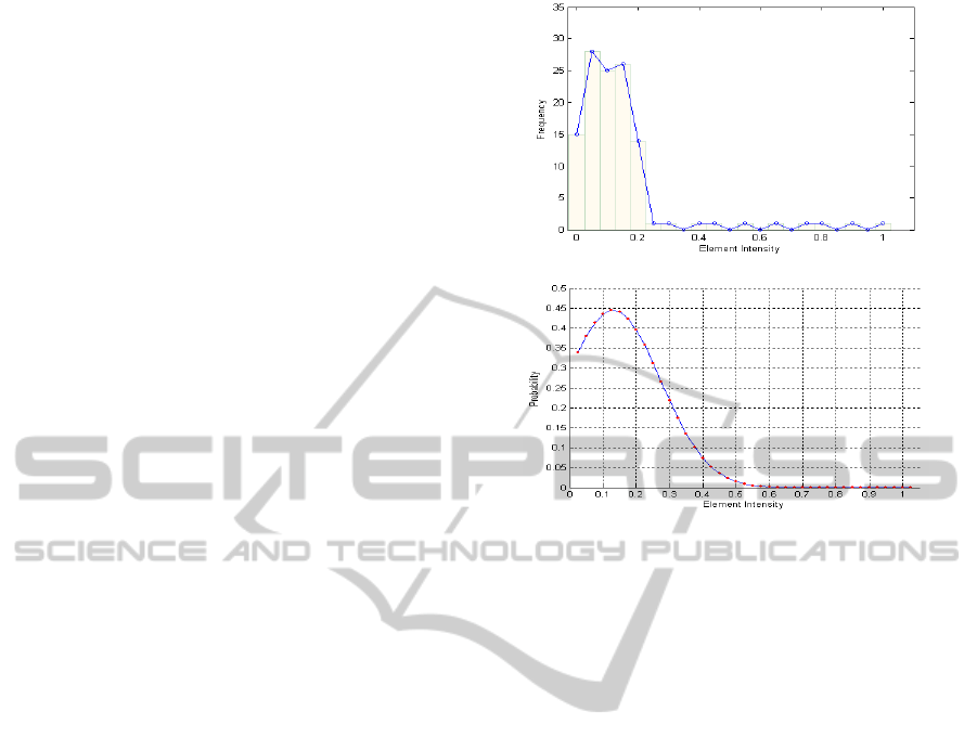
4.2 Gaussian Fitting and Element
Classification
Next, the normalized element value trajectory
alongside the regional attribute trajectory was fitted
by two separate Gaussian models. More specifically,
the recent history of each element,
)},,(,),1,,({ trErE
eleele
θ
θ
…
alongside the sum of
its regional attributes
)},,(,),1,,({ trErE
connconn
θ
θ
…
were modelled by the two Gaussian distributions.
The process of fitting the 251
st
element of the mesh
of figure 2, which is located in the upper left region
of the mesh, is shown in Figure 5 for
ele
E .
Finally, for each new frame, each of its elements
(a)
(b)
Figure 5: (a) Intensity histogram for the 251
th
element in
time (b) Fitted Gaussian probability distribution.
is classified to background or lung lobe region
according to the algorithm described in section III.
For the experiments, the learning rate parameter
α
was set to 0.002, while
η
= 2.5 gave the best
classifications. The results of the proposed method
on the EIT sequence of Figure 3(a) are shown in
Figure 6.
The effectiveness of the proposed method can be
seen from Figure 6. It shows that the probability
models were able to separate out the non-lung lobe
regions and picked out only areas of high
conductivity changes produced by the lobes without
producing outliers. With the proposed approach, the
use of regional information of each element as it
evolves through time permits the detection of the
globality of the change, recovering the correct
changes in the lobes.
5 CONCLUSIONS
The work proposes a novel, probabilistic method for
extracting regions of conductivity changes in EIT
lung images. The method involves modelling each
mesh element and its regional attribute as a time
series process fitted by a Gaussian model. Moreover,
a prior model of the background was also obtained
using anatomical structure of the thorax. The results
obtained from the different patient data show that
AUTOMATIC SEGMENTATION OF CONDUCTIVITY CHANGES IN ELECTRICAL IMPEDANCE TOMOGRAPHY
IMAGES
219

(a)
(b)
Figure 6: Segmentation results; image progression is from
left to right, top to bottom. Full-breath cycle is shown. (a)
proposed method (b) time-adaptive per-pixel MOG
method described in (Stauffer, 1999).
this new approach can be successfully applied to
automatically segment regions of conductivity
changes in EIT lung images. The procedure requires
minimal input fine-tuning and can capture the
dynamics of distinctly different regions in EIT
images. Further work involves the use of parallel
processing to speed up the segmenta-ion process so
that it can be used in real-time, for longer time
periods, and the extension of the framework to
segmentation on 3D meshes.
ACKNOWLEDGEMENTS
The authors gratefully acknowledge financial
support of this research through the grant provided
by the Engineering and Physical Sciences Research
Council (EPSRC) under Grant EP/E029868/1.
REFERENCES
Ackermann M.J., 1995. The Visible Human Project.
http://www.nlm.nih.gov, 1995. The authors gratefully
acknowledge financial support of this research through
the grant provided by the Engineering and Physical
Sciences Research Council (EPSRC) under Grant
EP/E029868/1.
Adler A. and Lionheart W. R. B., 2006. Uses and abuses
of EIDORS: An extensible software base for EIT.
Physiol Meas, 27:S25 {S42}
Brown B. H. and Seagar A. D., 1987. The Sheffield data
collection system, Clin. Phys. Physiol. Meas., 8,
(Suppl A) 91{97}.
Brown, B.H., 2003. Electrical impedance tomography
(EIT): a review, J Med Eng Technol. vol.:27, pp.97-
108.
Clay M.T. and Ferree T.C., 2002. Weighted regularization
in electrical impedance tomography with applications
to acute cerebral stroke. IEEE Trans. Med. Imaging,
Vol. 21, pp.629–37.
Frerichs I., 2000. Electrical impedance tomography (EIT)
in applications related to lung and ventilation: a review
of experimental and clinical activities. Physiological
Measurement, Vol. 21, no. 2, p. R1.
Frerichs, I., Scholz, J., and Weiler, N., 2006. Electrical
Impedance Tomography and its Perspectives in
Intensive Care Medicine. In J.L. Vincent (Ed.),
Yearbook of Intensive Care and Emergency Medicine,
Berlin: Springer, vol.10, pp. 437-444,
Molinari, M., 2003. High Fidelity Imaging in Electrical
Impedance Tomography. Ph.D. thesis, University of
Southampton, Southampton, United Kingdom.
Smallwood R. H., Hampshire A.R., Brown B.H., R. A.,
Primhak, Marven S. S., and Nopp P., 1999. A
comparison of neonatal and adult lung impedances
derived from EIT images. Physiological Measurement,
Vol. 20, pp. 401-413.
Stauffer M. C., and W. Grimson, 1999. Adaptive
background mixture models for real-time tracking.
IEEE Computer Society Conference on Computer
Vision and Pattern Recognition (Cat. No PR00149).
IEEE Comput. Soc. Part Vol. 2.
Sylvester J. and G. Uhlmann, G., 1986. A uniqueness
theory for an inverse boundary value problem in
electrical prospection. Commun. Pure Appl. Math.,
Vol.39, pp.91–112.
BIOSIGNALS 2011 - International Conference on Bio-inspired Systems and Signal Processing
220
