
A BAYESIAN METHOD FOR THE DETECTION OF EPISTASIS
IN QUANTITATIVE TRAIT LOCI
USING MARKOV CHAIN MONTE CARLO MODEL COMPOSITION
WITH RESTRICTED MODEL SPACES
Edward L. Boone
Department of Statistical Science and Operations Research, Virginia Commonwealth University, Richmond, Virginia, U.S.A.
Susan J. Simmons
1
, Karl Ricanek
2
1
Department of Mathematics and Statistics,
2
Department of Computer Science, University of North Carolina Wilmington
Wilmington, North Carolina, U.S.A.
Keywords:
Quantitative trait loci, Epistasis, Bayesian statistics, Markov chain Monte Carlo model composition.
Abstract:
Epistasis or the interaction between loci on a genome is of great interest to geneticists. Herein, a powerful
Bayesian method utilizing Markov chain Monte Carlo model composition approach using restricted spaces is
developed for identifying epistatic effects in Recombinant Inbred Lines (RIL). The method is verified through
a simulation study and applied to an Arabidopsis thaliana data set with cotyledon as the quantitative trait.
1 INTRODUCTION
Quantitative Trait Loci (QTL) analysis is concerned
with determining which region on a genome that ex-
plains or controls a quantitative trait. However, in
many instances an iteraction between regions or loci
may provide a better explanation for a trait than re-
gions having a strictly additive influence. This inter-
action between loci on a genome is known as epista-
sis. To study QTLs, organisms generated by recombi-
nant inbreeding are often used. Recombinant Inbred
Lines (RIL) are organisms that have been repeatedly
mated with siblings and themselves in order to create
a inbred line whose genetic structure is a combination
of the original parent organisms. These RILs provide
a mechanism to reduce environmental and individual
effects. Furthermore, these homozygous organisms
help simplify the search for the loci on the genome
has influence over a trait. This simplification is due
to fact that at each locus one does not need to know
the actual allele. Instead, one can track whether the
allele at a locus came from parent A or parent B. For
a complete review of RILs see (Broman, 2005).
Several methods have been developed to detect
and evaluate epistatic effects for continuous traits.
Multiple Interval Mapping (MIM) proposed by (Kao
et al., 1999) based on fitting a multiple regression
model that has both main effect terms as well as
interactions and employing a non-Bayesian search
method. (Carlborg, 2004) use a genetic algorithm
to search for the loci and epistatic effects. (Hansen
and Wagner, 2001) propose a theoretical framework
for higher order interactions. (Kao and Zeng, 2001)
use the framework of (Cockerham, 1954) to partition
the variance for known main and epistatic effects in
order to understand the contribution of each with no
search method. (Zeng et al., 2005) and (Wang and
Zeng, 2006) use (Cockerham, 1954) partition the vari-
ance when epistatic effects with multiple alleles are
present however no search method is presented in this
work either. (Hanlon and Lornez, 2005) use an op-
timization approach to find combinations of epistatic
effects that best represent the trait of interest based on
squared error distance.
To avoid this problem of model selection (Broman
and Speed, 2002) use Markov Chain Monte Carlo
Model Composition (MC
3
) to search for the main
effects (additive models) that contribute to the trait.
This procedure is a variant of reversible jump Markov
chain Monte Carlo by (Green, 1995). (Boone et al.,
71
L. Boone E., J. Simmons S. and Ricanek K..
A BAYESIAN METHOD FOR THE DETECTION OF EPISTASIS IN QUANTITATIVE TRAIT LOCI USING MARKOV CHAIN MONTE CARLO MODEL
COMPOSITION WITH RESTRICTED MODEL SPACES.
DOI: 10.5220/0003139200710078
In Proceedings of the 3rd International Conference on Agents and Artificial Intelligence (ICAART-2011), pages 71-78
ISBN: 978-989-8425-40-9
Copyright
c
2011 SCITEPRESS (Science and Technology Publications, Lda.)
2006) extend this to restricted model spaces to allow
for more loci than observations. (Yi et al., 2003), (Yi
et al., 2005), (Yi et al., 2007a), (Yi et al., 2007b) use
the MC
3
framework with various restrictions on the
model space to search for main and epistatic effects.
However, (Yi et al., 2003), (Yi et al., 2005), (Yi et
al., 2007a), (Yi et al., 2007b) and the R/qtlbim soft-
ware of (Yandell et al., 2007) do not require that the
main effect terms corresponding to the epistatic ef-
fects be present in the model. Furthermore, (Broman
and Speed, 2002), (Yi et al., 2003), (Yi et al., 2005),
(Yi et al., 2007a), (Yi et al., 2007b) and (Yandell et
al., 2007) employ information criteria such as AIC or
BIC as the basis for the MC
3
search. (Boone et al.,
2005) show that while BIC is an asymptotically cor-
rect approximation for posterior model probabilities,
in the low to moderate sample size case BIC performs
poorly.
The goal of this work is to explore a MC
3
algo-
rithm with restricted model spaces that require the
main effect terms corresponding to the epistatic be
present in the model. In addition, this article proposes
conditional activation probabilities as a tool to evalu-
ate epistatic effects in models where the correspond-
ing main effects are included. Furthermore, to avoid
the use of information criterion such as AIC or BIC
as the basis of the MC
3
search.
Current methods for assessing epistasis use fre-
qentist tests which are inherently model dependent.
This work uses activation probabilities (proposed by
(Boone et al., 2006) for use in QTLs), defined in Sec-
tion 2.2 for each of the main and epistatic effects to
determine the marginal posterior probability of each
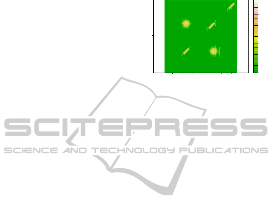
effect regardless of which model is chosen. Figure 1
shows an example heatmap of the activation probabil-
ities that may occur when epistasis is present. Activa-
tion probabilities along the diagonal correspond to the
main effect of the locus. The off diagonal activation
probabilities correspond to epistatic effects. Notice
that by looking along the diagonal the main effects
appear to be at locus 12, locus 26 and locus 35 as
the (12,12), (26, 26) and (35,35) regions have high
probability. Furthermore one can look at the off di-
agonal and see that loci 12 and 26 appear to have an
epistatic effect as well as noted by high probability in
the (12,26) region. However, loci 12 and 35 and loci
26 and 35 do not appear to have an epistatic effect due
to low probability in the regions common to (12,35)
and (26,35) on the heatmap.
Section 2 defines the model, basic search strat-
egy, activation probabilities and conditional activation
probabilities. Section 2.3 explains the neighborhood
definition and search strategy under restricted model
spaces. Section 3 gives a simulation study showing
0.0
0.2
0.4
0.6
0.8
1.0
5 10 15 20 25 30 35
5
10
15
20
25
30
35
Locus
Locus
Figure 1: Simulated heatmap of activation probabilities for
main effect and epistatic effects. Activation probabilities
along the diagonal correspond to main effects and off diag-
onal correspond to epistatic effects.
the efficacy of the method for detecting both main ef-
fects and two-way interaction effects. Section 4 con-
siders the Arabidopsis Thaliana as an example. The
dataset for this model organism has 158 lines of RIL
and 38 markers (loci) and cotelydon opening angle is
the quantitative trait of interest.
2 BAYESIAN MODEL SEARCH
2.1 Model Definition
Let y
i
be the quantitative trait for the i
th
observation.
For eahc of the p loci l
1
,l
2
,...,l
p
the parentage of the
allele is recorded as A if the allele came from parent
A and B if the allele came from parent B. However,
in some instances the allele is not determined which
needed to be reflected in the analysis. For the i
th
ob-
servation and locus l
j
this information can be coded
into X
ij
as:
X
ij
=
1, allele l
j
is from parent A
−1, allele l
j
is from parent B
0, allele l
j
is undetermined
(1)
Here the X
ij
correspond to the main effects. For the
epistatic effects (two-way interaction) this produces
the interaction between loci l
j
and l
k
as:
X
ij
X
ik
=
1, alleles l
j
and l
k
from same parent
−1, alleles l
j
and l
k
from different parents
0, allele l
j
or l
k
is undetermined
(2)
Using a traditional first order model with a two-
way multiplicative interaction terms the model is de-
ICAART 2011 - 3rd International Conference on Agents and Artificial Intelligence
72

fined as:
y
i
= µ+
p
∑
j=1
β
j
X
ij
I
P
c
(l
j
) +
∑
k< j
β
jk
X
ij
X
ik
I
P
c
(l
j
)I
P
c
(l
k
) + ε
i
.
(3)
where ε
i
∼ N(0,σ
2
c
), P
c
is the set of loci l
j
in
model M
c
, and I
P
c
is an indicator function that takes
the value 1 if l
j
∈ P
c
and 0 otherwise. Here β
j
cor-
responds to the main effect of locus l
j
and β
jk
is the
epistatic effect between loci l
j
and l
k
.
2.2 Bayesian Model Averaging
In a model space M with |M | models, the posterior
probability of model M
c
given the data D can be com-
puted via Bayes’ Theorem:
P(M
c
|D ) =
P(M
r
)P(D |M
c
)
∑
|M |
t=1
P(M
t
)P(D |M
t
)
. (4)
The marginal probability of the data D given model
M
c
, P(D |M
c
) is involved in computing (4) and can be
calculated using:
P(D |M
c
) =
Z
P(θ
c
|M
c
)P(D |θ
c
,M
c
)dθ
c
, (5)
where θ
c
is the parameter vector corresponding to
model M
c
. Evaluating the integral in (5) can be com-
plicated. Approximations such as the Laplace ap-
proximation and the approximationbased on Schwarz
Bayesian Information Criterion (BIC) could be em-
ployed. However, in the linear model case, as in equa-
tion (3), where the coefficient vector for model M
c
,
β
c
∼ N(µ
c
,V
c
) and σ
2
c
∼ Inv−χ
2
(ν,λ) prior is used,
an analytic expression for (5) is:
P(D |µ
c
,V
c
,ν,X
c
,M
c
) =
Γ
ν+n
2
(νλ)
ν
2
π
n
2
Γ
ν
2
|I + X
c
V
c
X
′
c
|
1/2
× [λν+ (Y −X
c
µ
c
)
′
× (I + X
c
V
c
X
′
c
)
−1
× (Y −X
c
µ
c
)]
−
ν+n
2
, (6)
where µ
c
and V
c
are the mean and variance, respec-
tively, and ν and λ are the degrees of freedom, and lo-
cation parameter, respectively. This work will employ
(6) for computing (5) versus any information criterion
based approximations.
In cases where the model space is sufficiently
large, calculating (5) for each model is computation-
ally infeasible. A stochastic search through the model
space can be performed using a metropolis-hastings
approach. For more on metropolis-hastings sampling
see (Chib and Greenberg, 1995), (Bolstad, 2010).
This can be accomplished by constructing neighbor-
hoods around the current model M
c
. Typically, the
neighborhoods nbd(M
c
) consist of all models with
one additional term than model M
c
and all models
with one less term than model M
c
. For a candidate
model M
t
∈nbd(M
c
) the probability, α, of acceptance
of model M
t
is given by.
α = min
1,
P(M
t
)P(D |M
t
)
P(M
c
)P(D |M
c
)
q(M
t
|M
c
)
q(M
c
|M
t
)
, (7)
where q(M
t
|M
c
) is the probability that the candidate
model is M
t
is selected for consideration given the
current state is model M
c
. Note the neighborhood
structure mentioned above is not appropriate when
the main effect terms are required to be in the model
whenever an epistatic term is in the model. (Yi et al.,
2003), (Yi et al., 2005), (Yi et al., 2007a), (Yi et al.,
2007b) and (Yandell et al., 2007) allow the neighbor-
hood to be all models with one main effect term more
or less than M
c
and all models with one epistatic effect
more or less than M
c
. Since they do not require than
when an epistatic term is in the model that the corre-
sponding main effect terms be in the model as well,
this is a reasonable neighborhood structure however
it is different than the structure proposed here. They
also further propose that the neighborhoods could in-
clude only loci that are near to current locus on the
genome.
Once the posterior model probabilities have been
computed activation probabilities can be used to as-
sess the impact of predictor X
j
and can be computed
via:
P(β
j
6= 0|D ) =
|M |
∑
c=1
P(β
j
6= 0|D ,M
c
)P(M
c
|D ). (8)
Activation probabilities are different from the tradi-
tional p-value in that largevaluesindicate significance
versus small values. In addition, activation probabili-
ties do not depend on a specific model as do p-values.
The activation probabilities can be calculated via MC
3
as defined in section 2.3.
Activation probabilities will have a problem de-
tecting two-way interactions when the main effect
terms are required to be in the model in order for the
two-way interaction term to be present. This induces
the following inequalities:
P(β
jk
|D ) ≤ P(β
j
|D ) (9)
P(β
jk
|D ) ≤ P(β
k
|D ).
Hence, using the standard activation probabilities for
two-way interaction effects will produce probabilities
that are damped. In order to amplify the activation
probabilities of the two-way interaction effects one
A BAYESIAN METHOD FOR THE DETECTION OF EPISTASIS IN QUANTITATIVE TRAIT LOCI USING
MARKOV CHAIN MONTE CARLO MODEL COMPOSITION WITH RESTRICTED MODEL SPACES
73

can use conditional activation probabilities. Condi-
tional activation probabilities can also be obtained by:
P(β
jk
6= 0|β
j
6= 0,β
k
6= 0,D ) (10)
=
P(β
jk
6= 0,β
j
6= 0,β
k
6= 0|D )
P(β
j
6= 0,β
k
6= 0|D )
,
provided that P(β
j
6= 0,β
k
6= 0|D ) > 0. In practice
one should only consider conditional activation prob-
abilities when both P(β
j
|D ) and P(β
k
|D ) are consid-
erably large. In cases where P(β
j
|D ) or P(β
k
|D ) are
small then unreasonably large inflations to the condi-
tional activation probabilities will occur and hence the
result in incorrect inferences.
2.3 Restricted Model Space
A simple approach to defining the neighborhoods of
a model M
c
is to include all models that add an ad-
ditional term or drop an existing term. However, this
violates a model that require both main effect terms
need to be present in the model in order for the cor-
responding two-way interaction to be added. Further-
more, the model need not contain all interaction terms
possible. Notice this creates a large model space.
For the first order models with p predictors the size
of the model space is 2
p
. However with the addi-
tion of interaction terms, the size grows considerably
more. In a dataset with 30 loci, a full model with all
first order terms and two-way interaction terms will
have 465 terms. This can be prohibitively large for
most datasets and algorithms. If the model space is
restricted to r < p predictors and the corresponding
epistasis terms, then any model considered will not
have nearly as many terms. If r is chosen wisely, then
the researcher can ensure that each model under con-
sideration has sufficient degrees of freedom to be es-
timated.
Furthermore, cases where linear dependencies ex-
ist among the predictors estimation can be compli-
cated. One approach to address this issue is to assign
P(M
c
) = 0 to all models where linear dependencies
exist among the predictors. Hence removing all mul-
ticollinear models from consideration. Any time there
are multicollinear terms an index will need to be cre-
ated in order to keep track of any aliased terms. This
aliasing can cause problems when there is a large ef-
fect size for the aliased terms.
The use of restricted model spaces allows for the
assessment of all candidate variables, however it re-
stricts the number of candidate variables that may be
simultaneously considered in a single model. (Yi et
al., 2003), (Yi et al., 2005), (Yi et al., 2007a), (Yi et
al., 2007b) and (Yandell et al., 2007) use two restric-
tions one for the number of main effect terms and one
for the number of epistatic terms allowed in the model
simultaneously. They also give a simple guideline to
determine the size of each restriciton. They suggest
to choose the restriction r = m+ 2
√
m where m is the
a priori expected number of main effects. Similarly
the same formula can be employed where m is the ex-
pected number of epistatic effect.
To search through the restricted model space,
MC
3
can be employed using equation (7). Note that
q(M
t
|M
c
) must be determined to move through the
sample space. Let nbd(M
c
) be all models with one
main effect term more, one valid interaction term
more, one main effect term less and one interaction
term less than model M
l
. Denote adding a main ef-
fect term as AMT, adding an interaction effect term as
AIT, dropping a main effect term as DMT and drop-
ping an interaction effct term as DIT. The probility of
each of these actions depends on the attributes of the
current model M
c
. Let γ
c
and φ
c
be the number of
main effect terms and number of interaction terms in
M
c
, respectively. In order to ensure that all models
in nbd(M
c
) are equally likely, the probability of each
action, AMT, AIT, DMT and DIT need to be deter-
mined. Let Ω = {AMT, AIT,DMT,DIT} be an action
space. Once these probabilities have been calculated,
the following procedure allows for each of the models
in nbd(M
c
) to be sampled to be candidate model. First
determine, P(AMT), P(AIT), P(DMT) and P(DIT),
and choose an action with the corresponding proba-
bility. Then select with equal probability a model that
is in nbd(M
c
) and corresponds to the action. This pro-
cedure ensures that all models in nbd(M
c
) have equal
probability. Having all models in nbd(M
c
) equally
likely will be necessary in computing q(M
c
|M
t
).
For γ
c
= 0, only a main effect term may be added
since no interaction terms are in the model. Hence the
probability distribution for Ω is:
P(AMT) = 1, P(DMT) = 0,
P(AIT) = 0,P(DIT) = 0. (11)
For γ
c
= 1, the one of the p−1 main effect terms
not in the model may be added or the one main effect
term in the model may be droped and no interaction
terms are allowed in this model. Hence the probabil-
ity distribution for Ω is:
P(AMT) =
p−1
p
,P(DMT) =
1
p
,
P(AIT) = 0,P(DIT) = 0. (12)
For 2 ≤ γ
c
≤ r, no restrictions are involved.
Hence, all actions in Ω are allowed. Hence, the prob-
ICAART 2011 - 3rd International Conference on Agents and Artificial Intelligence
74

ability distribution for Ω is:
P(AMT) =
p−γ
c
p+
γ
c
2
!
, P(AIT) =
γ
c
2
!
−φ
c
p+
γ
c
2
!
,
P(DMT) =
γ
c
p+
γ
c
2
!
, P(DIT) =
φ
c
p+
γ
c
2
!
.
(13)
For γ
c
= r, due to the restriction that no more than
r main effect terms may be in a model at a single time,
no main effect terms may be added. However, main
effect terms may be dropped and interaction terms
may be added or dropped. Hence, the probability dis-
tribution for Ω is:
P(AMT) = 0, P(AIT) =
r
2
−φ
r
r
2
+ k
,
P(DMT) =
r
r
2
+ r
,P(DIT) =
φ
c
r
2
+ r
.(14)
Since each model in nbd(M
c
) is equally likely
to be sampled, q(M
t
|M
c
) can easily be formed. For
example, let M
t
and M
c
be such that γ
t
= γ
c
+ 1
where γ
t
< r and γ
c
> 2. Then this corresponds
to the action AMT and the probability of candi-
date model M
t
given that the current model is M
c
is one out of the number of models in nbd(M
c
),
specifically, q(M
t
|M
c
) =
p+
γ
c
2
−1
and simi-
larly q(M
c
|M
t
) =
p+
γ
t
2
−1
. Hence the ratio of
the probability of candidate models for this case is:
q(M
t
|M
c
)
q(M
c
|M
t
)
=
p+
γ
t
2
p+
γ
c
2
.
3 SIMULATION STUDY
To validate this approach, loci information from Ara-
bidopsis thaliana Bay-0 × Shadara was used. Fig-
ure 2 illustrates the genetic map of the Arabidopsis
thaliana Bay-0 × Shadara,which has five chromo-
somes and on each chromosome each locus where the
parentage of the allele has been determined is marked.
There was a total of 38 loci used for this simulation
study and 158 lines.
To assess the ability of the method to detect both
main effects and epistatic effects a simulation study
Figure 2: Genetic map of the Arabidopsis Thaliana Bay-0
by Shadara.
was conducted. Using the loci matrix from the Ara-
bidopsis thaliana dataset two loci X
A
and X
B
were ran-
domly selected from the possible loci and the follow-
ing model was used to generate the data:
y
i
= δX
Ai
+ δX
Bi
+ δX
Ai
X
Bi
+ ε
i
, (15)
where δ is the effect size, ε
i
∼ N(0, 1). Each dataset
contained a sample size of 158 observations. Effect
sizes of 0, 1/2, 1, 3/2, 2, 5/2, 3, 7/2, 4, 9/2 and 5
were considered. Each of these effect sizes was re-
peated 10 times.
Using the data set and the method proposed the
following probabilties were calculated: P(X
A
|D ),
P(X
B
|D ), P(X
AB
|D ) and P(X
AB
|X
A
,X
B
,D). These
were calculated for 100 simulated data sets. Using
the following prior distributions β
j
∼ N(0,200) and
σ
2
∼ χ
2
(1) for the model parameters and P(M
i
) is
uniform over the all models subject to the restric-
tion of r = 10. For each simulated data set a chain
of 16,000 samples were taken from the posterior dis-
tribution of the models, with the first 1,000 samples
discarded as burn-in samples. The activation prob-
abilities were calculated using the remaining 15,000
samples.
Figure 3 show boxplots the main effect activation
probabilities versus the effect size from the simulated
datasets. Notice that for effect sizes of 0 and 1/2
the activation probabilities are low indicating that not
much evidence exists for the main effect at that locus.
However, for effect sizes at and above 1 the activa-
tion probabilites are quite high, typically above 0.8.
It should be noted that activation probabilities are not
associated with the idea of a p-value and hence can-
not be interpreted as such. Furthermore, the choice
of cutoff values for activation probabilities and what
is deemed statistically significant, in the Type I and
Type II error sense, has not been studied. However,
we should notice that the activation probabilities for
effect sizes at and above 1 are much larger than those
when the effect size is 0. Hence, one could feel con-
A BAYESIAN METHOD FOR THE DETECTION OF EPISTASIS IN QUANTITATIVE TRAIT LOCI USING
MARKOV CHAIN MONTE CARLO MODEL COMPOSITION WITH RESTRICTED MODEL SPACES
75

fident that the locus is important for influencing the
observed trait.
0 0.5 1 1.5 2 2.5 3 3.5 4 4.5 5
0.0 0.2 0.4 0.6 0.8 1.0
Effect Size
Activation Probabilities
Figure 3: Boxplots of main effect activation probabilities
for effect sizes 0, 1/2, 1, 3/2, 2, 5/2, 3, 7/2, 4, 9/2 and 5
using simulated data sets.
Figure 4 show boxplots for activation probabili-
ties of the epistatic effects and the conditional activa-
tion probabilities for epistatic effects versus the effect
size. Notice that in both plots that both the activa-
tion probabilities and the conditional activation prob-
abilities are low for effect sizes 0 and 1/2 indicating
that the epistatic effect of the two loci have no mini-
mal effect on the observed trait. However, notice that
for effect sizes larger than 1 the conditional activation
probabilities are considerably higher than the stan-
dard activation probabilities. Again there has been no
studies of cutoff values for activation probabilities nor
conditional activation probabilities. Looking at both
the activation probabilities and conditional activation
probabilities with reference to effect size 0 one could
feel confident that the two loci work in combination
to influence the observed trait.
0 0.5 1 2 4
0.0 0.2 0.4 0.6 0.8
Effect Size
Activation Probability
0 0.5 1 2 4
0.0 0.2 0.4 0.6 0.8
Effect Size
Conditional Activation Probability
Figure 4: Boxplots of epistatic effect activation proba-
bilities (left) and conditional activation probabilities for
epistatic effects (right) for effect sizes 0, 1/2, 1, 3/2, 2,
5/2, 3, 7/2, 4, 9/2 and 5 using 100 simulated data sets per
effect size. Dashed line at 1/2 is for reference.
4 EXAMPLE
The Arabidopsis thaliana is a model plant for genetic
experiments in that it is easily genetically manipu-
lated. The response of interest is the angle cotyledon
opening for 158 lines; the values range between 0 and
180. The cotyledon is the is the first embryonic leaves
on a seedling plant. The wider the opening angle the
more viable the mature plant.For each line at each of
the chromosomal locations (markers) a value of 1 or -
1 corresponding to whether the marker at that location
came from parent A or parent B, respectively. With
this data and using an unrestricted model space the
largest model would have 741 terms. Hence, many
models are not able to be fit. By restricting the model
space to r = 10 the largest model would have 55 terms
and thus, all models have enough observations to be
estimated.
To determine if any aliasing between the main
effects and interaction terms occured the data was
screened. This screening showed that no interaction
terms are aliased with any main effect term. Hence,
conclusions about the main effect terms will not be
confounded with any epistatic effects. An additional
screen of the data was performed to determine if there
is aliasing between any interaction effects. Aliased in-
teraction effects were noted for consideration during
posterior inferences.
For this example, the exact marginal posterior
probability of the data given model M
c
was computed
using equation (6) and the proposed MC
3
method with
restricted model space was utilized. For each model
under consideration the prior distributions for the
model parameters were defined as: β
ij
∼ N(0,200)
for all j and β
jk
∼ N(0,200) for all interaction terms
jk in model i; for σ
2
, λ = 1 and ν = 1 are used. Note
that when ν = 1 the Inv −χ
2
ν
has infinite mean and
variance. Hence, should be relatively uninformative.
For each model M
c
where multicollinearity does not
occur, the prior probability P(M
c
) is chosen uniform
across this space. Thus, a priori, no model is preferred
over another.
Using the restriction r = 10, 25 chains of 11,000
were run with a burn in of 1,000 samples using
overdispersed starting models resulting in 250,000
samples. The number of visits to model M
c
was
recorded and the probability of model given the data
P(M
c
|D) is estimated as the number of visits to model
M
c
divided by the length of the chain. The proba-
bilities appeared to converge after 15 chains, indicat-
ing convergence. Using these probabilities the activa-
tion probabilities P(β
j
6= 0|D ) are computed for each
main and epistatic effect. Figure 5 shows a heat map
of epistatic probabilities. Notice that the highest acti-
ICAART 2011 - 3rd International Conference on Agents and Artificial Intelligence
76

vation probability locus on the heat map is at locus 18
(ATHCHIB2) and no epistatic, off diagonal, effects
have high activation probability.
0.0
0.1
0.2
0.3
0.4
0.5
0.6
0.7
5 10 15 20 25 30 35
5
10
15
20
25
30
35
Locus
Locus
Figure 5: Heat map of epistatic probabilities.
The activation probabilities for the 3 highest
loci, ATHCHIB2, MSAT5-9 and MSAT5-22 are as
follows: P(ATHCHIB2|D ) = 0.741, P(MSAT5 −
9|D ) = 0.481 and P(MSAT5 − 22|D ) = 0.445.
This suggests that the following epistatic effects
should be considered: ATHCHIB2 × MSAT5 −
9, ATHCHIB2 × MSAT5 − 22 and MSAT5 −
9 × MSAT5 − 22. Previous studies have shown
ATHCHIB2 to be a locus associated with cotely-
don opening (Boone et al., 2006). Hence the re-
sults agree with biological expectations. In order to
more accurately locate the locus associated with cote-
lydon opening a dense map of genes near ATHCHIB2
should be undertaken.
Table 1: Activation probabilities and conditional activation
probabilities of epistatic effects between locus l
j
and locus
l
k
.
l
i
l
j
P(l
ij
|D ) P(l
ij
|l
i
,l
j
,D )
ATHCHIB2 MSAT5-9 0.070 0.243
ATHCHIB2 MSAT5-22 0.061 0.191
MSAT5-9 MSAT5-22 0.062 0.135
5 DISCUSSION
The proposed method for detecting epistasis has the
ability to determine which main effects as well as
which two-way interaction effects are present in a
dataset as evidenced by the simulation study. The
method was applied to the Arabidopsis thaliana data
and no epistatic effects were found with respect to
cotyledon opening angle. However, the known lo-
cus for controlling cotyledon opening was detected,
ATHCHIB2. The search method was employed in a
situation where the number of parameters in the full
model far exceeded the number of observations. The
search was done in a manner that allowed for suffi-
cient degrees of freedom for each model under con-
sideration.
A study of epistatic models which do not require
the first order terms to be present should be consid-
ered as well. This may allow for better detection of
epistatic effects as the model search does not need to
first add a main effect in order to later include the
epistatic term. In this case the model space would
be reduced by 2
p
models. However, if all other in-
teraction terms are equally likely to be added to the
model, the Metropolis-Hastings step may have low
acceptance probability and convergence of the MC
3
algorithm may be slow. In addition, any loci that have
effects that are not in interaction with other loci may
not be detected. Hence, reducing the utility of the
method.
Caution should be used when using restricted
model spaces. The method works best when it is be-
lieved that only a few loci control the trait of interest.
In cases where it is believed that a large number of
loci control the trait of interest, especially when this
exceeds the restriction on the model space, then the
search method maybe come very ineffective at assess-
ing both the main effect as well as the epstatic effects.
Since the models at the restriction boundary will have
high posterior model probabilites it may be difficult
to move through regions of lower probability towards
even more probable models. In most cases in genetics
it is believed that only a few loci control the trait of
interest.
REFERENCES
Broman, K. W. (2005) The Genomes of Recombinant In-
bred Lines Genetics, 169, 1133-1146.
Broman, K. W. and Speed, T. P. (2002) A model selection
approach for the identification of quantitative trait loci
in experimental crosses. J.R. Statist. Soc. B, 64, 641-
656.
Bolstad, W. M. (2010) Understanding Computational
Bayesian Statistics. John Wiley, New York. ISBN 0-
470-04609-8
Boone, E. L., Ye, K. and Smith, E. P. (2005) Assessment of
two approximation methods for computing posterior
model probabilities. Computational Statistics & Data
Analysis, 48, 221-234.
Boone, E. L., Simmons, S. J., Ye, K., Stapleton, A. E.
(2006) Analyzing quantitative trait loci for the Ara-
bidopsis thaliana using Markov chain monte carlo
model composition with restricted and unrestricted
model spaces. Statistical Methodology, 3, 69-78.
A BAYESIAN METHOD FOR THE DETECTION OF EPISTASIS IN QUANTITATIVE TRAIT LOCI USING
MARKOV CHAIN MONTE CARLO MODEL COMPOSITION WITH RESTRICTED MODEL SPACES
77

Carlborg, O., Andersson, L. and Kinghorn, B. (2000) The
Use of a Genetic Algorithm for Simultaneous Map-
ping of Multiple Interacting Quantitative Trait Loci
Genetics, 155, 2003-2010.
Chib, S. and Greenberg, E. (1995) Understanding the
MetropolisHastings Algorithm. American Statisti-
cian, 49, 327335.
Cockerham, C. (1954) An extension of the concept of parti-
tioning hereditary variance for the analysis of covari-
ances among relatives when epistasis is present. Ge-
netics, 39, 859-882.
Green, P. J. (1995) Reversible jump Markov chain Monte
Carlo computation and Bayesian model determina-
tion. Biometrika, 82, 711-732.
Hanlon, P. and Lorenz, A. (2005) A computational method
to detect epistatic effects contributing to a quantitative
trait. J. Thoer. Biol., 235, 350-364.
Hansen,T. F. and Wagner, G. P. (2001) Modeling genetic
architecture : a multilinear theory of gene interaction.
Theor. Popul. Biol, 59, 61-86.
Kao, C. H., Zeng, Z. B. and Teasdale, R. D. (1999) Multiple
Interval Mapping for Quantitative Trait Loci. Genet-
ics, 152, 1203-1216.
Kao, C. H. and Zeng, Z-B. (2002) Modeling Epistasis
of Quantitative Trait Loci Using Cockerham’s Model.
Genetics, 160, 1243-1261.
Wang, T. and Zeng, Z.-B. (2006) Models and partition of
varieance for quantitative trait loci with epistasis and
linkage disequilibrium. BMC Genetics, 7, 9.
Yandell, B. S., Mehta, T., Samprit, B., Shriner, D.,
Venkataraman, R., Moon, J. Y., Neeley, W. W., Wu,
H., von Smith, R. and Yi, N. (2007) R/qtlbim:
QTL with Bayesian Interval Mapping in experimen-
tal crosses. Bioinformatics, 23, 641-643.
Yi, N., Xu, S. and Allison D. B. (2003) Bayesian Model
Choice and Search Strategies for Mapping Interacting
Quantitative Trait Loci Genetics, 165, 867-883.
Yi, N., Yandell, B. S., Churchill, G. A., Allison, D. B.,
Eisen, E. J., and Pomp, D. (2005) Bayesian model
selection for genome-wide epistatic quantitative trait
loci analysis. Genetics, 170, 1333-1344.
Yi, N., Samprit, B., Pomp, D. and Yandell, B. S. (2007)
Bayesian Mapping of Genomewide Interacting Quan-
titative Trait Loci for Ordinal Traits Genetics, 176,
1855-1864.
Yi, N., Shriner, D., Samprit, B., Mehta, T., Pomp, D. and
Yandell, B. S. (2007) An efficient Bayesian model se-
lection approach for interacting quantitative trait loci
models with many effects. Genetics, 176, 1865-1877.
Zeng, Z-B., Wang, T. and Zou, W. (2005) Modeling quanti-
tative trait loci and interpretation of models. Genetics,
169, 1711-1725.
ICAART 2011 - 3rd International Conference on Agents and Artificial Intelligence
78
