OPTIMISING CLASSIFIERS FOR THE DETECTION OF
PHYSIOLOGICAL DETERIORATION IN PATIENT
VITAL-SIGN DATA
Sara Khalid, David A. Clifton, Lei Clifton and Lionel Tarassenko
Institute of Biomedical Engineering, Dept. of Engineering Science, University of Oxford
Old Road Campus, Roosevelt Drive, Oxford, OX3 7DQ, U.K.
Keywords: Novelty detection, Multi-class classification, SVM, MLP.
Abstract: Hospital patient outcomes can be improved by the early identification of physiological deterioration.
Automatic methods of detecting patient deterioration in vital-sign data typically attempt to identify devia-
tions from assumed “normal” physiological condition. This paper investigates the use of a multi-class ap-
proach, in which “abnormal” physiology is modelled explicitly. The success of such a method relies on the
accuracy of data annotations provided by clinical experts. We propose an approach to estimate class labels
provided by clinicians, and refine those labels such they may be used to optimise a multi-class classifier for
identifying patient deterioration. We demonstrate the effectiveness of the proposed methods using a large
data-set acquired in a 24-bed step-down unit.
1 INTRODUCTION
Adverse events in patient condition are often pre-
ceded by physiological deterioration evident in vital-
sign data (Buist et al., 1999), and it is well-
understood that patient outcomes can be improved
by detecting this deterioration sufficiently early
(NPSA, 2007). Machine learning techniques have
been shown to be able to detect such physiological
deterioration by analysing vital-sign data acquired
from patient monitors connected to acutely ill hospi-
tal patients, such as Parzen window estimators (Ta-
rassenko, 2005).
A large number of manual methods (Smith, 2008)
have been developed to allow clinicians to identify
patient deterioration on the general ward, based on
periodically-collected vital sign data, typically ac-
quired every two to four hours.
Both manual and automatic methods typically
perform novelty detection (or one-class classifica-
tion), in which deviations from some assumed
“normal” behaviour are identified. This is a com-
mon approach to the condition monitoring of critical
systems (Tarassenko, 2009), for which large num-
bers of examples of “normality” exist, but where
there are comparatively too few examples of system
failure to construct a multi-class classifier, in which
known failure conditions are explicitly modelled.
However, should sufficient examples of patient
deterioration be available, a multi-class approach
may be taken. It is assumed a priori that, given
sufficient examples of system failure, a multi-class
classifier will outperform a one-class classifier due
to the inclusion of more information in the classifier
(Bishop, 2006). This paper describes an investiga-
tion in which a large data-set of patient vital-sign
data was acquired during a clinical study such that a
multi-class approach to identifying patient deteriora-
tion may be taken. For this to be successful, accu-
rate class labels for the data are required. We inves-
tigate the reliability of class labels provided by clini-
cians, and propose methods to (i) estimate and refine
those labels automatically, and (ii) use the resultant
labels to optimise a multi-class classifier for detect-
ing patient deterioration.
2 ESTIMATING
CLINICAL LABELS
Obtaining accurate class labels for large, multivari-
ate data-sets of vital signs is particularly difficult.
The data-set considered in the investigation de-
scribed by this paper, for example, was four-
425
Khalid S., Clifton D., Clifton L. and Tarassenko L..
OPTIMISING CLASSIFIERS FOR THE DETECTION OF PHYSIOLOGICAL DETERIORATION IN PATIENT VITAL-SIGN DATA.
DOI: 10.5220/0003138904250428
In Proceedings of the International Conference on Bio-inspired Systems and Signal Processing (BIOSIGNALS-2011), pages 425-428
ISBN: 978-989-8425-35-5
Copyright
c
 2011 SCITEPRESS (Science and Technology Publications, Lda.)

dimensional, comprising heart rate (HR), breathing
rate (BR), peripheral arterial oxygen saturation
(SpO
2
), and the arithmetic mean of systolic and
diastolic blood pressures (the systolic-diastolic aver-
age, or SDA), was acquired from 332 patients in a
step-down unit, and contains over 18,000 hours of
patient data (Tarassenko, 2005). It is impractical for
clinical experts to annotate such a large data-set in
its entirety.
The approach taken with the data-set was to de-
termine retrospectively which periods of patient data
exceeded standard “medical emergency team”
(MET) criteria (Smith, 2008). The latter are stan-
dard thresholds on each vital sign that, if exceeded,
should result in the clinical review of the patient.
Periods of patient data that exceeded the MET crite-
ria for at least four minutes were shown to a panel of
clinicians, who then determined which periods were
due to artefact (such as a sensor becoming detached
from the patient), and which were sufficiently ab-
normal to require patient review. We here term the
latter class labels of “abnormal” patient condition
C
2
, and will refer to examples of “normal” patient
condition to have class label C
1
.
As vital signs can take more extreme values
during periods of abnormal physiology, the distribu-
tions of data from periods labelled C
2
have heavier
tails than the distributions of data from “normal”
patients. However, there is significant overlap be-
tween the distributions of data from the two classes.
Additionally some types of physiological abnormal-
ity are not represented in the data-set as frequently
as other types; e.g., apnoea and bradycardia (low BR
and HR, respectively) are under-represented in com-
parison with tachypnoea and tachycardia (high BR
and HR, respectively). We found that this imbal-
ance leads to a linear classifier trained using such
data successfully classifying the majority of the
more well-represented tachypnoea and tachycardia
data, while misclassifying the under-represented
apnoea and bradycardia data.
Similarly, a non-linear classifier trained using the
original labels incorrectly includes the distribution
of bradycardia and apnoea data within its decision
boundary, and hence misclassifies test data from this
region of data space as belonging to class C
1
.
The remainder of this paper investigates methods
for refining class labels C
1
and C
2
, such that they
may be used to construct a multi-class classifier that
successfully classifies under-represented types of
“abnormal” data. We will illustrate the procedure
using bivariate analysis, such that the decision
boundary of a classifier may be examined. The
application to the full multivariate data-set (e.g., 4-
dimensional in this example) is considered in
Section 4.
3 REFINING CLINICAL LABELS
TO OPTIMISE THE
CLASSIFIER
The left-hand plot of Figure 1 shows all of the data
from the two classes in the bivariate space of HR
and BR. Clusters of C
2
data corresponding to ap-
noea, tachypnoea, bradycardia, and tachycardia may
be seen in the figure, although data from class C
1
often overlap with those clusters. Intuitively, we
wish to increase the separation between the two
classes such that a classifier trained using those
labels results in a decision boundary that correctly
classifies data from all modes of class C
2
. We pro-
pose a method for doing so using an estimate of the
probability density function (pdf) of the entire data-
set.
3.1 Defining a Multivariate
Distribution to Estimate Labels
We approximated the pdf of the whole data-set using
a Parzen windows estimator (Bishop, 2006), after
reducing the size of the data-set to 400 prototype
patterns using k-means clustering with k = 400 clus-
ter centres. The covariance σ
2
of the 400 kernels in
the pdf was set using the heuristic proposed in
(Bishop, 2006). Given some data-point x’, its den-
sity κ
x
= p(x’) defines a contour on the pdf. We then
define a probability P[κ
x’
] as follows:
P




=










(1)
where κ
m
= max[ p ], the density at the mode of the
pdf, p. Thus P[κ
x’
] is the probability mass contained
by integrating the pdf from its highest point down to
the probability density contour κ
x’
. This represents
the probability that some random data-point x dis-
tributed according to p will take a density value
higher than density value κ
x’
; i.e., P[κ
x’
] ≡ P[ p(x) ≥
κ
x’
]. Thus, as x’ varies throughout the data space,
its probability density will vary over the range
[0 κ
m
], and thus P[κ
x’
] will vary over the range [0 1]
correspondingly.
We define a threshold T on P[κ
x’
], and consider
which data have P[κ
x’
] ≥ T for varying values of T.
As described above, we expect data that lie fur-
thest from the mode of the distribution of the whole
BIOSIGNALS 2011 - International Conference on Bio-inspired Systems and Signal Processing
426

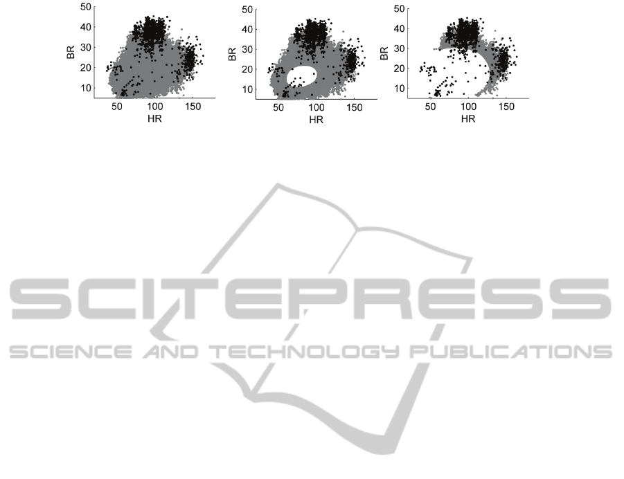
Figure 1: Data from classes C
1
and C
2
shown in grey and black, respectively. The left-hand plot shows all data from classes
C
1
and C
2
. Data x from C
1
are shown where P[κ
x
] ≥ T, for T = 0, 0.5, and 0.9 from left to right, respectively, as described in
Section 3.1.
data-set to take largest value of P[κ
x’
], and hence as
T is increased, the proportion of data that have P[κ
x’
]
≥ T will decrease. This effect is shown in Figure 1,
in which increasing the value of T causes fewer data
to lie above the threshold.
This suggests that we could use such a threshold
T to estimate the clinical labels for “abnormal” data;
i.e., those from class C
2
.
3.2 Optimising a Classifier using a
Threshold on the Multivariate
Distribution
In order to increase the separation between “normal”
and “abnormal” data used for training a classifier,
we can refine the C
1
and C
2
class labels provided by
clinicians using the following rules:
i. Define the training set of “normal” data to
be

∈

| P






(2)
ii. Define the training set of “abnormal” data
to be

∈

| P






(3)
In order to examine the effect of varying values of
the threshold T, 75% of the data from C
2
that obeyed
the above selection criterion were drawn at random,
and an equal number of data from class C
1
were
drawn at random. All remaining data from class C
2
were used as test data, and an equal number of data
randomly selected from the unused data from class
C
1
were used as test data.
The procedure involving threshold T was used to
process the training data only, and thus results ob-
tained using the test data are independent of T, giv-
ing an accurate representation of the system’s per-
formance when classifying previously-unseen data.
This is required in order to allow a fair comparison
with classification performance obtained without
using the proposed method.
Figure 2 shows the misclassification rates
obtained when non-linear classifiers (multi-layer
perceptron with a single layer of hidden units, or
MLP, in this example) were compared over N = 50
experiments. We note that the results are shown
based on the test data, and that the classifier archi-
tecture was selected using 10-fold cross-validation.
It may be seen from the figure that, as the value
of the threshold T is increased from 0 to 1, the num-
ber of false-positive misclassifications decreases
while the number of false-negative misclassifica-
tions increases. This is because the “normal” train-
ing data (the refined version of class C
1
) cover a
larger locus as T increases. Conversely, the “ab-
normal” training data (the refined version of class
C
2
) cover a smaller locus as T increases. Thus, the
resulting decision boundary of the classifier be-
comes less sensitive to abnormality with increasing
T, because the classifier is trained with an increas-
ingly large cluster of “normal” data and a decreas-
ingly small set of clusters of “abnormal” data.
The figure shows that for T ≈ 0.4, these misclas-
sifications are minimised, which represents the “op-
timal” value of the threshold T for processing the
training data obtained from this data-set.
Similar results were obtained when applying the
proposed technique with a support vector machine
(SVM) classifier. Figure 3 shows the decision
boundary obtained using an SVM both using the
original C
1
and C
2
labels, and the “refined” labels
created by using the procedure described previously.
It may be seen that the SVM decision boundary
obtained without application of the proposed method
covers large areas of data space that correspond to
physiological deterioration; e.g., the region that
corresponds to tachypnoea (at BR > 30 rpm) for HR
≈ 75 bpm. In comparison, the SVM decision boun-
dary obtained after application of the proposed me-
thod more closely describes the locus of “normal”
data, in the centre of the data space, and accurately
separates the four modes of data-space that corres-
pond to apnoea, tachypnoea, bradycardia, and
tachycardia.
OPTIMISING CLASSIFIERS FOR THE DETECTION OF PHYSIOLOGICAL DETERIORATION IN PATIENT
VITAL-SIGN DATA
427

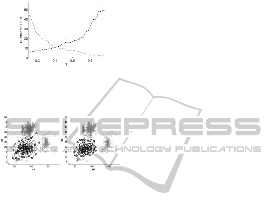
Figure 2: Misclassification performance evaluated using
the test set, as threshold T is varied. Mean false-positive
(FP, shown by a solid line) and false-negative (FN, shown
by a dotted line) errors over a range of N = 50 experiments
for each value of T, with a confidence interval on each
value shown at ± 1 standard deviation from the mean.
Figure 3: Using original (left-hand plot) and refined (right-
hand plot) C
1
and C
2
labels to construct a SVM classifier.
The SVM produces a decision boundary shown by the
black line, with support vectors indicated by circles.
4 DISCUSSION AND FUTURE
WORK
We have presented a method of (i) estimating clini-
cal labels, and (ii) using the technique to refine ex-
isting labels such that a classifier may be trained that
better separates “normal” data from “abnormal”
data, when compared with classifiers that do not use
the proposed technique.
While this paper has presented the results of a
bivariate analysis, such that the decision boundaries
of classifiers may be examined and compared, the
procedure should be applied in the dimensionality of
the original data space; in the example considered by
this paper, the data-set is 4-dimensional (HR, BR,
SpO
2
, and SDA). The thresholding procedure is
performed using the high-dimensional pdf, and so
the proposed method of estimating and refining
clinical labels is equally applicable to optimising
classifiers in the original high-dimensional data-
space.
A further advantage of the proposed method is
that, as described in Section 2, as the value of the
threshold T is increased, the distribution of data with
probability P exceeding that threshold tends towards
the distribution of data labelled as being class C
2
by
clinicians. While there is no equal substitute for the
annotations of clinical experts, it is impractical for a
panel of experts to review 18,000 hours of continu-
ous data. As described in Section 2, the C
2
labels
were obtained as being a subset of those periods that
exceeded univariate MET criteria for periods of at
least four minutes, and so even these are not “gold
standard” labels of the entire data-set. However,
being able to estimate such labels is useful: the pro-
cedure can be applied to further, unlabelled data-sets
in order to estimate their class C
2
labels. Thus, it
may be possible to obtain automatically labelled
data-sets from large unlabelled data-sets, which
would previously require the use of an unsupervised
classification approach, such as the one-class
method described in Section 1, and in (Tarassenko,
2005) and (Tarassenko, 2009).
REFERENCES
Buist, M. D., Jarmolowski, E., Burton, P. R., Bernard, S.
A., Waxman, B. P., Anderson, J., 1999: Recognising
Clinical Instability in Hospital Patients Before Cardiac
Arrest or Unplanned Admission to Intensive Care.
Med. J. Australia, Vol. 171 8–9.
NPSA, 2007. National Patient Safety Association: Safer
Care for Acutely Ill Patients: Learning from Serious
Accidents. Tech. Rep
Tarassenko, L., Hann, A., Patterson, A., Braithwaite, E.,
Davidson, K., Barber, V., Young, D., 2005: Multi-
parameter Monitoring for Early Warning of Patient
Deterioration. Proc. 3rd IEE Int. Seminar on Medical
Applications of Signal Processing, London, 71-6.
Smith, G. B., Prytherch, D. R., Schmidt, P. E., Feather-
stone, P. I.,2008: Review and Performance Evaluation
of Aggregate Weight “Track and Trigger” Systems. J.
Resuscitation, Vol. 77, 170-179.
Tarassenko, L., Clifton, D. A., Bannister, P. R., King, S.,
King, D., 2009: Novelty Detection. In: Staszewski,
W. J., Worden, K. (eds), Encyclopaedia of Structural
Health Monitoring, Wiley.
Bishop, C. M., 2006.: Pattern Recognition and Machine
Learning. Springer-Verlag.
BIOSIGNALS 2011 - International Conference on Bio-inspired Systems and Signal Processing
428