ACCURATE LATENCY CHARACTERIZATION FOR VERY

LARGE ASYNCHRONOUS SPIKING NEURAL NETWORKS

Mario Salerno, Gianluca Susi and Alessandro Cristini

Institute of Electronics, Rome University at Tor Vergata, Rome, Italy

Keywords: Neuron, Spiking Neural Network (SNN), Latency, Event-driven, Plasticity, Threshold, Neuromorphic,

Neuronal group selection.

Abstract: The simulation problem of very large fully asynchronous Spiking Neural Networks is considered in this

paper. To this purpose, a preliminary accurate analysis of the latency time is made, applying classical

modelling methods to single neurons. The latency characterization is then used to propose a simplified

model, able to simulate large neural networks. On this basis, networks, with up to 100,000 neurons for more

than 100,000 spikes, can be simulated in a quite short time with a simple MATLAB program. Plasticity

algorithms are also applied to emulate interesting global effects as the Neuronal Group Selection.

1 INTRODUCTION

A significant class of simulated neuromorphic

systems is represented by Spiking Neural Networks

(SNN), in which the neural activity consists of

spiking events generated by firing neurons (E. M.

Izhikevich, J. A. Gally, G. M. Edelman, 2004), (W.

Maas, 1997). In order to consider realistic models,

the simulation of the inner dynamics of the neurons

can be very complex and time consuming (E. M.

Izhikevich, 2004). Indeed, accurate neuron models

consist of complex systems of non-linear differential

equations, so that any actual simulation is

computationally convenient only in the case of quite

small networks. On the other hand, only in the case

of large networks, a number of interesting global

effects can be investigated, as the well known

Neuronal Group Selection, introduced by Edelman

(G. M. Edelman, 1987). In order to consider the

simulation of large networks, it is important to

introduce simplified models, in which any single

neuron be able to produce a class of firing patterns

quite similar to those of the biological counterpart.

In this paper, a proper SNN model will be

introduced, based on some fundamental properties of

neurons. The proposed model is able to simulate

large neuromorphic maps, up to 100,000 neurons.

A basic problem to realize realistic SNN

concerns the apparently random times of arrival of

the synaptic signals (G.L. Gernstein, B. Mandelbrot,

1964). Many methods have been proposed in the

technical literature in order to properly

desynchronizing the spike sequences; some of these

consider transit delay times along axons or synapses

(E. M. Izhikevich, 2006), (S. Boudkkazi, E. Carlier,

N. Ankri, O. Caillard, P. Giraud, L. Fronzaroli-

Molinieres and D. Debanne, 2007). A different

approach introduces the spike latency as a neuron

property depending on the inner dynamics (E. M.

Izhikevich, 2007). Thus, the firing effect is not

instantaneous, as it occurs after a proper delay time

which is different in various cases. In this work, we

will suppose this kind of desynchronization as the

most effective for SNN simulation.

Spike latency appears as intrinsic continuous

time delay. Therefore, very little sampling times

should be used to carry out accurate simulations.

However, as sampling times grow down, simulation

processes become more time consuming, and only

short spike sequences can be emulated. The use of

the event-driven approach can overcome this

difficulty (D’Haene, B. Schrauwen, J. V.

Campenhout and D. Stroobandt, 2009), since

continuous time delays can be used and the

simulation can easily proceed to large sequence of

spikes. Indeed, simulations of more than 100,000

spikes are possible by this method in a quite short

computing time.

In the proposed model, classical learning

algorithms can easily be applied in order to get

proper adjustment of the synaptic weights. In such a

116

Salerno M., Susi G. and Cristini A..

ACCURATE LATENCY CHARACTERIZATION FOR VERY LARGE ASYNCHRONOUS SPIKING NEURAL NETWORKS.

DOI: 10.5220/0003134601160124

In Proceedings of the International Conference on Bioinformatics Models, Methods and Algorithms (BIOINFORMATICS-2011), pages 116-124

ISBN: 978-989-8425-36-2

 2011 SCITEPRESS (Science and Technology Publications, Lda.)

way, adaptive neural networks can be implemented

in which proper plasticity rules are active. In

presence of input signals, the simulation of the

whole network shows the selection of neural groups

in which the activity appears very high, while it

remains at a quite low level in the regions among

different groups. This auto-confinement property of

the network activity seems to remain stable, even

when the considered input is terminated.

The paper is organized as follows: description

and simulation of some basic properties of the

neuron, such as threshold and latency; introduction

of the simplified model on the basis of the previous

analysis, description of the network structure,

plasticity algorithm, input structure, simulation

results and performance tests.

2 LATENCY

CHARACTERIZATION

Different kinds of neurons can be considered in

nature, with special and peculiar properties (S.

Ramon y Cajal, 1909-1911). On the other hand,

many models have been introduced and compared in

terms of biological plausibility and computational

cost. Antipodes are the Integrated and Fire (L.

Lapicque, 1907) and the Hodgkin-Huxley Model

(A.L. Hodgkin, A.F. Huxley, 1952), the first one

characterized by low computational cost and low

fidelity, while the second is a quite complete

representation of the real case.

In the latter case, the model consists of four

differential equations describing membrane

potential, activation of Na+ and K+ currents, and

inactivation of Na+ current (E. M. Izhikevich, 2007).

From an electrochemical point of view, the neuron

can be characterized by its membrane potential V

In the simulation starting case, the neuron lies in

its resting state, i.e. V

= V

rest

(Resting Potential),

until an external excitation is received.

The membrane potential varies by integrating the

input excitations. Since contributions from outside

are constantly added inside the neuron, a significant

accumulation of excitements may lead the neuron to

cross a threshold, called firing threshold TF (E. M.

Izhikevich, 2007), so that an output spike can be

generated.

However, the output spike is not immediately

produced, but after a proper delay time called

latency (R. FitzHugh, 1955). Thus, the latency is the

delay time between exceeding the membrane

potential threshold and the actual spike generation.

From a physiological point of view, such a delay

time is usually attributed to the slow charging of the

dendritic tree, as well as to the action of the A-

current, namely the voltage-gated transient K+

current with fast activation and slow inactivation.

The current activates quickly in response to a

depolarization and prevents the neuron from

immediate firing. With time, however, the A-current

inactivates and eventually allows firing (E. M.

Izhikevich, 2007). This phenomenon is affected by

the amplitudes and widths of the input stimuli and

thus rich dynamics of latency can be observed,

making it very interesting for the global network

desynchronization.

It is quite evident that latency concept strictly

depends on an exact definition of the threshold level.

However, strictly speaking, the true threshold is not

a fixed value, as it depends on the previous activities

of the neuron, as shown by the Hodgkin-Huxley

equations (A.L. Hodgkin, A.F. Huxley, 1952).

Indeed, a neuron is similar to a dynamical system, in

which any actual state depends on the previous ones.

The first work addressing the threshold from a

mathematical point of view was FitzHugh (R.

FitzHugh, 1955), who defined the Quasi Threshold

Phenomenon (QTP). A finite maximum latency is

defined, but neither a true discontinuity in response

nor an exact threshold level are considered. Indeed,

with reference to the squid giant axon model, it has

been pointed out that the membrane fluctuations for

experimental observations or insufficient accuracy

for the simulators, make not possible to establish an

exact value of the threshold. To this purpose, in

figures 1a and 1b, it is shown that the neuron

behaviour is very sensitive with respect to small

variations of the excitation current.

Nevertheless, in the present work, an appreciable

maximum value of latency will be used. This value

is determined by simulation and applied to establish

a reference threshold point. When the membrane

potential becomes greater than the threshold, the

latency appears as a function of V

. To this purpose,

proper simulations have been carried out for single

neurons.

3 SINGLE NEURON

SIMULATIONS

Significant latency properties will be analysed in this

section. To this purpose, the NEURON Simulation

Environment (http://www.neuron.yale. edu/neuron/)

has been used, a tool for quick development of

ACCURATE LATENCY CHARACTERIZATION FOR VERY LARGE ASYNCHRONOUS SPIKING NEURAL

NETWORKS

117

Figure1: Change of membrane potential, caused by two

current pulses of 0.01 ms applied to the initial resting state

at t = 0. The amplitudes are 0.64523 nA (fig. 1a) and

0.64524 nA (fig. 1b). The behaviours, obtained by the

simulator NEURON, appear very sensitive with respect to

the current amplitude and justify the name “All-Or-None

law”, adopted in neuroscience in these cases.

Figure 2: Instantaneous variation of ΔV

for an impulsive

current injected I

ext

realistic models for single neurons, on the basis of

Hodgkin-Huxley equations.

In the field over the threshold level, the latency

can directly be related to input current pulses,

received as stimuli from spikes generated by afferent

neurons. Since the instantaneous variations of

membrane potential (

ΔV

) appear almost linear

with respect to the related current pulses, the latency

can also be represented as a function of the

membrane potential. Note that, starting from the

resting state (Vrest = -65 mV), an excitatory pulse of

1 nA (0.01 ms time width) corresponds to

ΔV

= 10

mV .

Three significant cases have been simulated,

using the integration step of 0.00125 ms and the

current pulse width of 0.01 ms.

α) Case of Single Excitatory Current Pulses

Starting from the resting state, an input current pulse

of proper amplitude, able to cause output spike after

a proper latency time, has been applied. Simulating a

set of examples, with current pulses in the range [

0.64524 ÷ 10 ] nA , the latency as a function of the

pulse amplitude, or else of the membrane potential

, has been determined. The latency behaviour is

shown in Fig. 3, in which it appears decreasing, with

an almost hyperbolic shape. The threshold level

corresponds to the pulse amplitude equal to 0.64524

nA , with the maximum latency of 10.6313 ms .

Pulses with less amplitudes are under the threshold

level, so that no output spikes are more obtained in

these cases.

Figure 3: Latency as a function of the membrane potential

(or else of the current amplitude Iext , equivalently).

β) Case of Two Excitatory Current Pulses

Starting from the resting state, after a first input

current pulse, able to cause an output spike, a second

pulse has been applied in the latency interval, in

order to analyse the corresponding latency speed up

in the firing process. As the first pulse is of fixed

amplitude (equal to 0.64524 nA), the overall latency

is a function of the second pulse amplitude (varying

in the range [ 0.001 ÷ 5 ] nA) and of the time interval

Δ, between the two excitatory current pulses.

In fig. 4, the behaviours of the overall latency

time, i.e. the time between the first pulse and the

output spike, in function of the second pulse

amplitude, are shown, for different values of Δ. Note

that the overall latency always decreases with the

second pulse amplitude. However, while the effect

of the second pulse is quite relevant for low values

of Δ, it becomes almost irrelevant when Δ is high,

i.e. almost equal to the value of the latency

corresponding to the first pulse only.

γ) Case of a First Excitatory and a Second

Inhibitory Current Pulse.

Starting from the resting state, after a first input

current pulse, able to cause an output spike, a second

pulse has been applied in the latency interval, after

the

time interval Δ. The second pulse is negative, so

BIOINFORMATICS 2011 - International Conference on Bioinformatics Models, Methods and Algorithms

118

Figure 4: Set of behaviours corresponding to excitatory-

excitatory stimuli. Each curve represents the overall

latency in function of the second stimulus amplitude, for a

fixed time interval Δ between the two stimuli. The effect is

greater in the case of low values of Δ.

that an inhibitory effect is produced. As the first

pulse is of fixed amplitude (equal to 3.0 nA, which

ensures that the membrane potential is carried quite

over the threshold), the second one is of varying

amplitude (from -0.01 nA, until it be still possible to

appreciate the output spike).

Once the second pulse is applied, the main effect

is the generation of an action potential delay

increment, caused by the inhibitor pulse. The more

the inhibitor pulse is strong, the greater the delay

resulted in the generation of action potential. In

addition, more the inhibitor pulse is timely, greater

is the latency produced. Even in this case, the overall

latency is a function of the second pulse amplitude

(fig.5). It is worth to emphasize that, as the interval

between the two pulses becomes relatively large, the

influence of the inhibitor is cancelled.

Figure 5: Set of behaviours corresponding to excitatory-

inhibitory stimulation. Each curve represents the latency in

function of the inhibitory stimulus amplitude, for a fixed

time interval Δ between the two stimuli. The latency

variation is greater in the case of low values of Δ.

4 SIMPLIFIED NEURON MODEL

IN VIEW OF LARGE NEURAL

NETWORKS

In the simplified model, a number of normalized and

simplified quantities are introduced, to represent

their physical counterpart. The membrane potential

is represented by a normalized real positive number

S , said the inner state of the neuron, defining the

value S = 0 as the resting state. The firing threshold

corresponds to the value S

, so that the activity of

the neuron can properly be classified, as passive

mode if S < S

, and active mode if S > S

In active mode, the neuron is ready to fire, and

the latency is modelled by a real positive quantity t

called time-to-fire . To this purpose, a bijective

correspondence between the state S and t

introduced, called the firing equation. A simple

choice for the normalized firing equation is the

following one:

= 1 / ( S - 1 ) , for S > S

(1)

In the model, t

is a measure of the latency, as it

represents the time interval in which the neuron

remains in the active state. Thus, time-to-fire

decreases with time and, as it gets to zero, the firing

event occurs. If the normalized firing threshold S

chosen such that

= 1 +

(2)

the maximum value of time-to-fire is equal to

f,max

= 1 /

(3)

Equation (1) is a simplified model of the

behaviour shown in section 3, fig. 3. Indeed, as the

latency is a function of the membrane potential,

time-to-fire is dependent from the state S, with a

similar shape, like a rectangular hyperbola. The

simulated and the denormalized firing equation

behaviours are compared in fig. 6.

Figure 6: Comparison between the latency behaviour and

that of the denormalized firing equation. The two

behaviours present a shape similar to a rectangular

hyperbola.

ACCURATE LATENCY CHARACTERIZATION FOR VERY LARGE ASYNCHRONOUS SPIKING NEURAL

NETWORKS

119

In a similar way, it could easily be proved that

also the behaviours shown in fig.s 4 and 5 can

correctly be modelled by the proper use of the firing

equation. Indeed, it is important to stress that

equation (1) must be applied as a bijective relation.

Thus, in the case of more input pulses, the following

steps must be considered.

a) As the appropriate first input is applied, the

neuron enters in active mode, with a proper state S

and a corresponding time-to-fire t

f A

b) According to the bijective firing equation, as

time goes on,

f A

decreases to the value t

f B

= t

f A

- Δ

and the corresponding inner state S

increases to the

new value S

, until the second input is received.

c) After the interval Δ, the second input is

received. It is clear that now the new state

is to be

considered. The state S

is now affected by the input

and, the greater is Δ (in the interval 0 < Δ <

f A

), the

greater the corresponding value of S

. Thus, the

effect of the second input pulse becomes irrelevant

for great values of Δ.

This peculiar property proves the good validity

of the proposed model.

In the model, the firing event consists in the

generation of the output signal. When the firing

event occurs in a certain neuron, it is said a firing

neuron. The firing event consists of the following

steps.

A) Transmission of the firing signals through the

output synapses connected to the receiving neurons,

said burning neurons. In the proposed model, the

transmission is considered instantaneous, thus the

transmitted signals are impulses of amplitude equal

to the presynaptic weight, Pr.

B) Resetting the inner state S to the rest state S =

C) For each directly connected burning neuron k,

modification of its inner state S

= S

+ Pr Pw

(4)

in which Pw is the related postsynaptic weight of the

considered synapse.

Figure 7: Proposed model for the neuron.

It is evident that the model introduces a

modulated delay for each firing event. This delay

strictly depends on the inner dynamics of the neuron.

Time-to-fire and firing equation are basic

concepts to make asynchronous the whole neural

network. Indeed, if the firing equation is not

introduced, and time-to-fire is always equal to zero,

the fire event would be produced exactly when the

state S becomes greater than S

, and this would

happen at the same time for all the neurons reaching

their active modes. Thus, the behaviour of the whole

network would be synchronous. The definition of

time-to-fire as a continuous variable let the firing

process dependent on the way by which each firing

neuron has reached its active mode.

In the classical neuromorphic systems, neural

networks are composed by excitatory and inhibitory

neurons. In our model, the presynaptic weight P

are

chosen positive for excitatory and negative for

inhibitory neurons.

5 NETWORK STRUCTURE

The connection map of the neurons is defined

establishing for each firing neuron (in which the

firing event is produced) the burning neurons

directly connected to it by proper synapses, through

proper postsynaptic weights. It is evident that the

difference between firing and burning neurons is

only considered to define the related synapses and

the network topology. Indeed, any neuron can be

minded either firing or burning, whether it generates

or receives a spiking signal. The whole synapse

distribution can be stored in a general N x N matrix [

] , in which N is the total number of neurons.

Each entry of this matrix represents the post-

synaptic weight corresponding to a firing vs. a

burning neuron. If such a synapse is not present, the

entry is zero, and thus, as the synaptic connection

net among neurons is usual quite not complete, the

matrix [ P

] will be sparse. Moreover, for large

number of neurons, the complete N x N matrix

cannot easily be stored. Thus, proper sparse matrix

technique has been applied in the simulation

program, in order to optimise the memory

requirements.

Many network topologies could be implemented

by this technique. In the proposed simulation

program, the simple case of local like connections is

considered, as in the case of Cellular Neural

Networks (L.O.Chua, L.Yang, 1988) . Each firing

neuron is directly connected to a number of burning

neurons belonging to a proper neighbourhood. The

BIOINFORMATICS 2011 - International Conference on Bioinformatics Models, Methods and Algorithms

120

local connection maps are shown in fig.s 8 and 9,

where grids of excitatory (en) and inhibitory (in)

neurons are indicated. The following classes of

synapse kinds are defined: s

, s

, while

synapses s

are never present (the subscript e stands

for excitatory neuron, and i for inhibitory neuron).

Figure 8: Map of synapses s

, and s

; xn stands for

excitatory or inhibitory firing neuron, while en for

excitatory burning neurons.

As shown in the literature, greater

neighbourhood is applied for inhibitory neurons (G.

M. Edelman, 1987). Therefore, in the case of

synapses s

, inhibitory burning neurons are not

neighbouring to the related excitatory firing

counterpart. Note that fig.s 8 and 9 refer to the case

of minimum neighbourhood.

Figure 9: Map of synapses s

; en stands for excitatory

firing neuron, while in for inhibitory burning neurons.

6 PLASTICITY RULES

Plasticity consists in the proper variation of the post-

synaptic weights P

, according to the neuron

dynamics. All the P

weights are bounded from a

minimum to a maximum value, and are always

positive quantities. The classical Hebb rule was

proved not to be quite suitable to properly model the

complex plasticity behaviour of natural nervous

system. In this paper, three plasticity effects have

been implemented, according to (G. M. Edelman,

1987).

Exponential decay: all postsynaptic weights are

decreased to the minimum value in an exponential

way with proper time constant.

Heterosynaptic enhancement: when a burning

event occurs from a certain synapse, the

postsynaptic weight is increased to the maximum

value, in function of previous burnings on the same

neuron, in a specified time window (heterosynaptic

window) from other synapses.

Homosynaptic enhancement: when a burning

event occurs from a certain synapse, the

postsynaptic weight is increased to the maximum

value, in function of previous burnings on the same

neuron and from the same synapse, occurred in a

specified time window (homosynaptic window).

The growing rates (increase, decrease) related to

hetero and homosynaptic rules are properly chosen.

7 SIMULATION

The proposed neural paradigm has been

implemented in a simple MATLAB program. The

simulation method proceeds looking for the next

firing event occurring in the whole network. It can

be seen that the proposed model is not suitable for a

classical simulation procedure based on a specified

sampling time. Indeed, as small this sampling time is

chosen, two contiguous firing events are likely to

occur in the whole net, in a less time interval. Thus,

larger networks are simulated, smaller time intervals

can occur. Time continuity in the simulation is then

necessary, in particular for very fast dynamics. On

the other hand, the use of very little sampling times

can make very slow the simulation process.

Then, it is evident that event-driven simulation

method is quite suitable to the proposed neural

model. To this purpose, a proper matrix is

introduced in which all the active neurons are stored,

together with their time-to-fire values. Looking for

the lower time-to-fire, the next firing event is

identified in term of the firing neuron and the instant

of the event. Then, the active neuron matrix is

properly updated and the new time value is

identified in the event driven process. Therefore, the

simulation proceeds in a very fast way.

Network activity is based upon two steps.

en en en

en xn en

en en en

en xn en

en en en

in in in

in en in

in in in

in en in

in in in

ACCURATE LATENCY CHARACTERIZATION FOR VERY LARGE ASYNCHRONOUS SPIKING NEURAL

NETWORKS

121

1. Searching for the active neuron with the

minimum time-to-fire

2. Evaluation of the effects of the firing event to

all the burning neurons.

A necessary condition to maintain the activity is

that unless one neuron be active in every time. If this

is not the case, all the neurons are passive and the

activity is terminated.

Burning events can be classified in four classes.

a. Passive Burning. In this case a passive neuron

remains still passive after the burning event, i.e. the

inner state is always less than the threshold.

b. Passive to Active Burning. In this case, a

passive neuron becomes active after the burning

event, i.e. the inner state becomes greater than the

threshold, and the proper value of the time-to-fire

can be evaluated. This is possible only in the case of

excitatory firing neurons. The case α ) , analysed in

section 3, belongs to this class of burnings.

c. Active Burning. In this case an active neuron,

affected by the burning event, still remains active,

while the inner state can be increased or decreased

and the time-to-fire is properly modified. The cases

β ) and γ ), analysed in section 3, belong to this class

of burnings.

d. Active to Passive Burning. In this case an

active neuron comes back to the passive mode. This

is only possible in the case of inhibitor firing

neurons. The inner state decreases and becomes less

than the threshold. The related time-to-fire is

cancelled.

Since any firing event always makes passive the

firing neuron, the frequency of burnings of classes a)

and b) must be sufficiently high. Indeed, burnings of

class c) only modify the time evolution, and burning

of class d) reduces the global activity. On this basis,

many criteria can be introduced to evaluate the

activity level of the whole network.

A significant parameter by which the global

stability can be controlled is the presynaptic weight

which represents the firing signal amplitude for

each firing neuron in the net. Indeed, lower values of

lead to the reduction of total number of firing

neurons, up to the deadline of any activity. On the

contrary, higher values of P

let increase the firing

number, up to the saturation of the system. A quite

correct value of P

can be chosen considering the

number of synapses starting from a given firing

neuron (fan-out, f

). Since each firing event

produces the resetting of inner state S from S

(normalized threshold) to 0 , the value S

can be

thought distributed among all the synapses outgoing

the neuron. Thus, a useful choice is Pr = S

/ f

. This

choice was proved quite likely to guarantee the

network stability.

7.1 Input Structure

Input signals are considered quite similar to firing

spikes, though depending from external events.

Input firing sequences are connected to some

specific neurons through proper external synapses.

Thus, proper input burning neurons are chosen.

External firing sequences are multiplied by proper

postsynaptic weights in the burning process. Also

these weights are affected by the described plasticity

rules, thus the same inputs can be connected to

different burning neurons, showing different effects

in the various cases.

7.2 Simulation Tests

Several simulation tests have been carried out on the

proposed neural paradigm. In many cases, random

values for the postsynaptic weights have been

chosen as starting point for the simulation.

If proper input sequences are simulated, and if

the proposed plasticity rules are active, some

properties of the network evolution have been

verified, in particular the selection of specific neural

groups, in which the activity appears in a quite high

level, while it remains lower in the regions among

different groups. This auto-confinement property of

the network activity seems to remain stable, even if

the considered input is terminated.

As an example, we propose a neural network of

the following characteristics:

Number of excitatory neurons = 18060

number of inhibitory neurons = 2021

number of external sources = 25

The excitatory neurons are located in a

bidimensional grid. The size of the grid is 140 x 129.

Since a neighbourhood equal to 4 is chosen, a total

number of 1,608,220 postsynaptic weights is

implemented. As an initial choice, these weights

have been assigned in a random way, from a

minimum to a maximum value. In order to carry out

a network able to show an initial activity, proper

starting values for the states S have been assigned.

In this way, the initial number of active neurons was

equal to 2452.

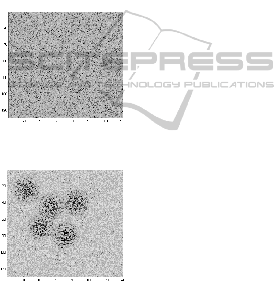
In fig. 10, the map of the network is represented,

in which every neuron is shown as a point. Clearer

points represent neurons in the cases of lower values

of their inner states S, while darker points refer to

the cases of higher S.

BIOINFORMATICS 2011 - International Conference on Bioinformatics Models, Methods and Algorithms

122

We present here the simulation parameters of the

network after a number of firings equal to 22518.

The normalized inner simulation time is equal to

116.5, where the number of active neurons is

reduced to 1096. The new neuron map is shown in

fig. 11, in which the activity of the network appears

not uniform, as that shown in fig. 10. Indeed, five

specific groups are now present, in which the most

of active neurons are grouped. The bounds of groups

are quite sharp and the activity in the regions among

them is near to zero.

Figure 10: Map of the neural network used in the

simulation test. Each point represents a single neuron.

Brighter points stand for low values of S , darker for

higher values. The map refers to the random initial

configuration, before processing.

Figure 11: The same map of fig. 10, after simulation. The

Neural Group Selection clearly appears.

The simulation parameters, involved in the

process from the initial map of fig. 10 to that of fig.

11, are the following ones:

Number of firing = 22,517

Number of burnings:

passive = 1,163,500

passive-to-active = 21,020

active = 568,891

active-to-passive = 1223

The parameters involved in the plasticity rules

are the following ones:

Number of etherosynaptic upgrading

= 39,469,900

Number of homosynaptic upgrading

= 2,341,430

Typical time performances of the simulation test

is about 11 minutes, on a Pentium dual core 2.5 GHz

(ram: 2GB).

8 CONCLUSIONS

Neural networks based on a very simple model have

been introduced. The model belongs to the class of

Spiking Neural Networks in which a proper

procedure has been applied to accounting for latency

times. This procedure has been validated by accurate

latency analyses, applied to single neuron activity by

simulation methods based on classical models. The

firing activity, generated in the proposed network,

appears fully asynchronous and the firing events

consist of continuous time sequences. The

simulation of the proposed network has been

implemented by an event-driven method, allowing

the possibility of simulating very large network by a

quite simple MATLAB procedure. The simulation

shows the appearance of the well known Neuronal

Group Selection, when proper input sequences and

proper plasticity rules are applied.

Future works in the field could be about the

stability analysis of the firing activity and of the

plasticity rules, in order to generate permanent

functional groups in the whole network. The results

related to the analysis of chaotic firing processes in

single groups seem also very promising.

REFERENCES

E. M. Izhikevich, J. A. Gally, G. M. Edelman, 2004:

“Spike-timing dynamics of neuronal groups”, 14:933–

944. Oxford University press.

ACCURATE LATENCY CHARACTERIZATION FOR VERY LARGE ASYNCHRONOUS SPIKING NEURAL

NETWORKS

123

W. Maas, 1997: “Networks of Spiking Neurons: The Third

Generation of Neural Network Models”. Elsevier

Science Ltd.

E. M. Izhikevich, 2004: “Which model to use for cortical

spiking neurons?” IEEE Transactions on neural

networks, Vol. 15

G. M. Edelman, 1987: “Neural Darwinism: The Theory of

Neuronal Group Selection”. Basic Books, New York.

G. L. Gernstein, B. Mandelbrot, 1964: “Random walk

models for the spike activity of a single neuron”.

Biophisical journal, Vol.4.

E. M. Izhikevich, 2006: “Polychronization: computation

with spikes”. Neural Computation 18, 18:245-282.

S. Boudkkazi, E. Carlier, N. Ankri, O. Caillard, P. Giraud,

L. Fronzaroli-Molinieres and D. Debanne, 2007:

“Release-Dependent Variations in Synaptic Latency: A

Putative Code for Short- and Long-Term Synaptic

Dynamics”.Neuron, volume 56, issue 6.

E. M. Izhikevich, 2007: “Dynamical Systems in

Neuroscience: The Geometry of Excitability and

Bursting”. The MIT press.

M. D’Haene, B. Schrauwen, J. V. Campenhout and D.

Stroobandt, 2009: “Accelerating Event-Driven

Simulation of Spiking Neurons with Multiple Synaptic

Time Constants”. Neural computation, apr. 21(4).

S. Ramon y Cajal, 1909, 1911: “Histologie du Systeme

Nerveux de l'Homme et des Vertebres, vol. I & II”.

L. Lapicque, 1907: “Recherches quantitatives sur

l’excitation électrique des nerfs traitée comme une

polarization”.

A. L. Hodgkin, A.F. Huxley, 1952: “A quantitative

description of membrane current and application to

conduction and excitation in nerve”, Journal of

Physiology, 117, 500-544.

R. FitzHugh, 1955: “Mathematical models of threshold

phenomena in the nerve membrane”. Bull.

Math.Biophysics

http://www.neuron.yale.edu/neuron/

L. O. Chua, L.Yang, 1988: “Cellular Neural Networks:

Theory”. IEEE Trans. Circuits Syst., vol. 35.

BIOINFORMATICS 2011 - International Conference on Bioinformatics Models, Methods and Algorithms

124