
EXTRACTION OF FUNCTION FEATURES
FOR AN AUTOMATIC CONFIGURATION
OF PARTICLE SWARM OPTIMIZATION
Tjorben Bogon
1,2
, Georgios Poursanidis
1
, Andreas D. Lattner
1
and Ingo J. Timm
2
1
Information Systems and Simulation, Institute of Computer Science and Mathematics
Goethe University Frankfurt, Frankfurt, Germany
2
Business Informatics I, University of Trier, Trier, Germany
Keywords:
Particle swarm optimization, Machine learning, Swarm intelligence, Parameter configuration, Objective func-
tion feature Computation.
Abstract:
In this paper we introduce a new approach for automatic parameter configuration of Particle Swarm Optimiza-
tion (PSO) by using features of objective function evaluations for classification. This classification utilizes a
decision tree that is trained by using 32 function features. To classify different functions we compute features
of the function from observed PSO behavior. These features are an adequate description to compare different
objective functions. This approach leads to a trained classifier which gets as input a function and returns a pa-
rameter set. Using this parameter set leads to an equal or better optimization process compared to the standard
parameter settings of Particle Swarm Optimization on selected test functions.
1 INTRODUCTION
Metaheuristics in stochastic local search are used in
numerical optimization problems in high-dimensional
spaces. For varying types of mathematical functions,
different optimization techniques vary w.r.t. the op-
timization process (Wolpert and Macready, 1997). A
characteristic of these metaheuristics is the configu-
ration of the parameters (Hoos and St
¨
utzle, 2004).
These parameters are essential for the efficient opti-
mization behavior of the metaheuristic but depend on
the objective function, too. An efficient set of param-
eters influences the optimization in speed and perfor-
mance. If a good parameter set is selected, an ade-
quate solution will be found faster compared to a bad
configuration of the metaheuristic. The choice of the
parameters is based on the experience of the user and
his knowledge about the domain or on empirical re-
search found in literature. This parameter settings,
called standard configurations, perform a not opti-
mal but an adequate optimization behavior for most
objective functions. An example for metaheuristics
is the Particle Swarm Optimization (PSO). PSO is
introduced by (Eberhart and Kennedy, 1995) and is
a population-based optimization technique which is
used in continuous high dimensional search spaces.
PSO consists of a swarm of particles which “fly”
through the search space and update their position by
taking into account their own best position and de-
pending on the topology, the best position found by
other particles. PSO is an example for the parameter
configuration problem. If the parameters are well cho-
sen, the whole swarm will find an adequate minimum
and focus on this solution. The swarm slows down
the velocity trying to get better values in the continu-
ous search space around this found solution. This ex-
ploitation can be on a local optimum especially if the
wrong parameter set is chosen and the swarm cannot
escape from this local minimum. On the other hand
the particles can never find the global optimum if they
are too fast and never focus. This swarm behavior de-
pends mainly on the chosen parameter and leads to
solutions of different quality.
One problem in choosing the right parameters
without knowledge about the objective function is to
identify relevant characteristics of the function which
can be used for a comparison among functions. The
underlying assumption is that, e.g., a function f
1
= x
2
and a function f
2
= 3x
2
+ 2 exhibit similar optimiza-
tion behavior if the same parameter set for a Particle
Swarm Optimization is used. In order to choose a
promising parameter set, functions must be compara-
51
Bogon T., Poursanidis G., D. Lattner A. and J. Timm I..
EXTRACTION OF FUNCTION FEATURES FOR AN AUTOMATIC CONFIGURATION OF PARTICLE SWARM OPTIMIZATION.
DOI: 10.5220/0003134500510060
In Proceedings of the 3rd International Conference on Agents and Artificial Intelligence (ICAART-2011), pages 51-60
ISBN: 978-989-8425-40-9
Copyright
c
2011 SCITEPRESS (Science and Technology Publications, Lda.)

ble with respect to certain objective function charac-
teristics.
We describe an approach to computing features of
the objective function by observing the swarm behav-
ior. For each function we seek for a parameter set
that performs better than the standard configuration
and provide this set as output class for supervised
learning. These data allow us to train a C4.5 deci-
sion tree (Quinlan, 1993) as classifier that computes
an adequate configuration for the Particle Swarm Op-
timization by using function features. Experimental
trials show that our decision tree classifies functions
into the correct classes in many cases. This classifica-
tion can be used to select promising parameter sets for
which the Particle Swarm Optimization is expected to
perform better in comparison to the standard configu-
ration.
This work is structured as follows: In section 2 we
describe other approaches pointing out the problem
of computing good parameter sets for a metaheuristic
and explain the Particle Swarm Optimization. Section
3 describes how to compute the features of a function
and thereby make the functions comparable. After
computing the features we describe our experimental
setup and the way to build up the decision tree. Sec-
tion 4 contains our experimental results for building
the parameter classes to select promising parameter
sets in PSO. The last section discusses our results and
describes issues for future work.
2 PARAMETER SETTINGS
IN METAHEURISTICS
The main difference between solving a problem with
exact methods or with metaheuristics is the quality
of the solution. Metaheuristics – for example, na-
ture inspired metaheuristics (Bonabeau et al., 1999)
– have no guarantee of finding the global optimum.
They focus on a point in the multidimensional search
space which results to the best fitness value depend-
ing on the experience of the past optimization per-
formance. This can be a local optimum, too. But
the advantage of the metaheuristic is to find an ade-
quate solution of a multidimensional continuous op-
timization problem in reasonable time (Talbi, 2009).
This performance depends on the configuration of
the metaheuristics and is an important fact of using
metaheuristics. One group of metaheuristics are the
population based metaheuristics. (Talbi, 2009) de-
fines population-based metaheuristics as nature in-
spired heuristics which handle more than one solution
at a time. With every iteration all solutions are re-
computed based on the experience of the whole pop-
ulation. Examples of population-based metaheuris-
tics are Genetic Algorithms which are an instance of
Evolutionary Algortihms, Ant Colony Optimization
and Particle Swarm Optimization. Different kinds of
metaheuristics exhibit varying performance on a spe-
cific kinds of problem types. They differ w.r.t. the
optimization speed and the solution quality. A meta-
heuristic’s performance is based on their configura-
tion. Finding a good parameter set is a non-trivial task
and often based on a priori knowledge about the ob-
jective function and the problem. Setting up a meta-
heuristic with standard parameter sets lets the opti-
mization find a decent solution but using a parameter
set which is adapted to the specific objective function
might even lead to better results. In this paper we
focus on PSO and try to find features characterizing
the objective function in order to select an adequate
parameter configuration for this metaheuristic. The
optimization behavior of the particles is based on the
objective function and we try identify relevant infor-
mation about the function. In the following section
we give a brief introduction to particle swarm opti-
mization.
2.1 Particle Swarm Optimization
Particle Swarm Optimization (PSO) is inspired by
the social behavior of flocks of birds and shoals of
fish. A number of simple entities, the particles, are
placed in the domain of definition of some function
or problem. The fitness (the value of the objective
function) of each particle is evaluated at its current
location. The movement of each particle is deter-
mined by its own fitness and the fitness of particles
in its neighborhood in the swarm. PSO was first in-
troduced in (Kennedy and Eberhart, 1995). The re-
sults of one decade of research and improvements to
the field of PSO were recently summarized in (Brat-
ton and Kennedy, 2007), recommending standards for
comparing different PSO methods. Our definition is
based on (Bratton and Kennedy, 2007). We aim at
continuous optimization problems in a search space
S defined over the finite set of continuous decision
variables X
1
, X
2
, . . . , X
n
. Given the set Ω of conditions
to the decision variables and the objective function
f : S → R (also called fitness function) the goal is to
determine an element s
∗
∈ S that satisfies Ω and for
which f (s
∗
) ≤ f (s), ∀s ∈ S holds. f (s
∗
) is called a
global optimum.
Given a fitness function f and a search space S the
standard PSO initializes a set of particles, the swarm.
In a D-dimensional search space S each particle P
i
consists of three D-dimensional vectors: its position
x
i
= (x
i1
, x
i2
, . . . , x
iD
), the best position the particle
ICAART 2011 - 3rd International Conference on Agents and Artificial Intelligence
52

visited in the past p
i
= (p
i1
, p
i2
, . . . , p
iD
) (particle
best) and a velocity v
i
= (v
i1
, v
i2
, . . . , v
iD
). Usually
the position is initialized uniformly distributed over S
and the velocity is also uniformly distributed depend-
ing on the size of S. The movement of each particle
takes place in discrete steps using an update function.
In order to calculate the update of a particle we need
a supplementary vector g = (g
1
, g
2
, . . . , g
D
) (global
best), the best position of a particle in its neighbor-
hood. The update function, called inertia weight, con-
sists of two parts. The new velocity of a particle P
i
is
calculated for each dimension d = 1, 2, . . . , D:
v
new
id
= w ·v
id
+ c
1
ε
1d
(p
id
−x
id
) + c
2
ε
2d
(g
d
−x
id
)
(1)
then the position is updated: x
new
id
= x
id
+ v
new
id
. The
new velocity depends on the global best (g
d
), particle
best (p
id
) and the old velocity (v
id
) which is weighted
by the inertia weight w. The parameters c
1
and c
2
pro-
vide the possibility to determine how strong a particle
is attracted by the global and the particle best. The
random vectors ε
1
and ε
2
are uniformly distributed
over [0, 1)
D
and produce the random movements of
the swarm.
2.2 Algorithm Configuration Problem
The general problem of configuring algorithms (algo-
rithm configuration problem) is defined by Hutter et
al. (Hutter et al., 2007) as finding the best tuple θ
out of all possible configurations Θ (θ ∈ Θ). θ rep-
resents a tuple with a concrete assignment of values
for the parameter of an algorithm. Applied to meta-
heurisitcs the configuration of the algorithm parame-
ters for a specific problem influences the behavior of
the optimization process. Different parameter settings
exhibit different performances at solving a problem.
The problem to configure metaheuristics is a super
ordinate problem and is analyzed for different kinds
of metaheuristics. In PSO the convergence of the
optimization depending on different parameter set-
tings and different functions are analyzed by (Trelea,
2003), (Shi and Eberhart, 1998) and (van den Bergh
and Engelbrecht, 2002). But these approaches focus
only on the convergence of the PSO but not on func-
tion characteristics and the relationship between the
parameter configuration and the function landscape.
Different approaches to solve this algorithm con-
figuration problem on metaheurisitcs are introduced:
One approach is to find sets of adequate parameters
which performs a good optimization on most different
types of objective functions. This “standard param-
eters” are evaluated on a preset of functions to find
a parameter set which leads to global good behavior
of the metaheuristic. In PSO standard parameter sets
are presented by (Clerc and Kennedy, 2002) and (Shi
and Eberhart, 1998). Some approaches do not present
a preset of parameters but change the values of the
parameters during the runtime to get a better perfor-
mance (Pant et al., 2007).
Another approach is introduced by Leyton-Brown
et al. They try to create features which describe the
underlying problem (Leyton-Brown et al., 2002) and
generate a model predicting the right parameters de-
pending on the classification. They introduce several
features which are grouped into nine groups. The fea-
tures include, among others, problem size statistics,
e.g. number of clauses and variables, and measures
based on different graphical representations. This
analysis is based on discrete search spaces because
on continuous search spaces it is not possible to set
adequate discrete values for the parameter configura-
tion which is needed by their appraoch.
Our problem is to configure an algorithm working
on continuous search spaces and offers infinite pos-
sibilities of parameter sets. To solve this challenge
we try, similar to Leyton-Brown et al., to train a clas-
sifier with features of the fitness function landscape
computed by observing swarm behavior. These fea-
tures are computed and combined with the best found
parameter set on the function to a training instance
(see figure 1). With a trained classifier at hands we
compute the features of the objective function prior
to the start of the optimization process. The classifier
– in our case a decision tree – classifies the function
and selects the specific parameter set that is expected
to perform better in the optimization process than us-
ing the standard parameters. In our first experiments,
which we understand as proof of concept, we choose
only a few functions which do not represent any spe-
cific types of function. We want to show that our
technique is able to identify functions based on the
swarm behavior provided features and thereby, select
the specific parameter configuration. In order to learn
the classifier which suggests the parameter configura-
tion, different function features are computed. These
features are the basis of our training instances.
3 COMPUTATION OF FUNCTION
FEATURES
Our computed features can be divided into three
groups. Each group implies a distinct way of collect-
ing information about the fitness topology of the ob-
jective function from particles. The first group Ran-
dom Probing describes features which are calculated
based on a random selection of fitness values and
provides a general overview of the fitness topology.
EXTRACTION OF FUNCTION FEATURES FOR AN AUTOMATIC CONFIGURATION OF PARTICLE SWARM
OPTIMIZATION
53
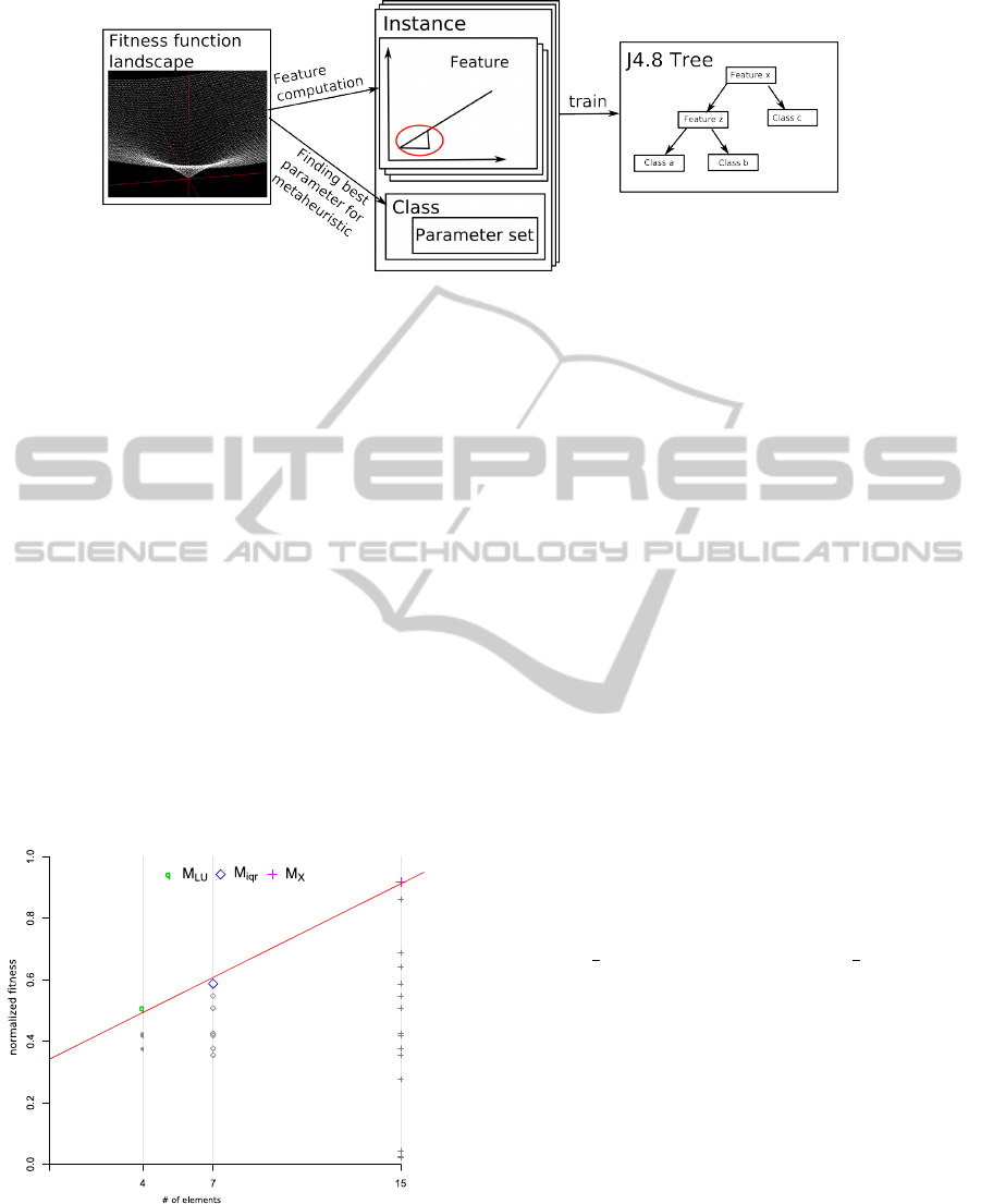
Figure 1: Process of building a classifier.
Distance-based features are calculated for the second
group Incremental Probing. They reflect the distribu-
tion of surrounding fitness values of some pivot parti-
cles. The third group of features utilizes the dynamics
of PSO to create features by using the changes of the
global best fitness within a small PSO instance. The
features are scale independent, i.e., that scaling the
objective function by constants will not affect the fea-
ture values. By this we imply that a configuration for
PSO leads to the same behavior on a function f as
it shows for its scaled function f
0
= α f + β, α > 0.
These three groups are based on each other which
means that the pivot particle for the second group is
taken from a particle of the first group to reduce the
computing time. Important for all these features are
the number of evaluations of the objective function.
The feature computation should be only a small part
of the whole optimization computation time.
Figure 2: Example of a random probing with the comutation
of µ
RP.Max
.
3.1 Random Probing
Random Probing defines features that are calculated
based on a set of k = 100 random particle positions
which are within the initialization range of the ob-
jective function (100 particles to get a short but ad-
equate description about the function window). Prob-
ing the objective function results in a distribution of
fitness values which is used to extract three features.
Trivial characteristics like mean and standard devi-
ation cannot be used as features since they are not
scale independent. That means, they will change their
value if the function is scaled by constants. In or-
der to create reliable features, the fitness values of all
points are evaluated and three sets of particles (includ-
ing their evaluation values) are created based upon
these values. The first set is denoted M
X
and con-
tains all fitness values of the randomly selected points.
The quartiles for the distribution of the fitness val-
ues are computed and the values between the upper
or lower quartile are joined into the second set. This
set is denoted M
iqr
. The third set M
LU
consists of the
fitness values which are between a lower and upper
boundary L and U. These boundaries are defined by
L = Q
1
+
1
2
(Q
M
−Q
1
) and U = Q
M
+
1
2
(Q
3
−Q
M
)
where Q
M
denotes the median and Q
1
, Q
3
denote
the lower and upper quartile of M
X
. For each set
M
X
⊃ M
iqr
⊃ M
LU
the number of elements is deter-
mined.
The feature Random Probing Min µ
RP.Min
is cal-
culated based on the linear model that fits the rela-
tionship between the number of values and the min-
imum fitness values in each set. The straight line of
the model is divided by the interquartile range of M
X
.
Similar to this the feature Random Probing Max is
based on the slope of the straight line that describes
the relationship of the number of elements and the
maximum value of each set M
X
⊃ M
iqr
⊃ M
LU
(see
figure 2). The slope divided by the interquartile range
of M
X
denoted by µ
RP.Max
is the second feature of
this group. Finally, for the feature Random Probing
ICAART 2011 - 3rd International Conference on Agents and Artificial Intelligence
54

Range denoted by µ
RP.Range
the spread, that is the
difference between the maximum and the minimum
value, in each set is computed. As for the other fea-
tures the slope is divided by the interquartile range of
M
X
. All features of this group are computed based on
the fitness values of the randomly selected points. For
each point the objective function is evaluated once,
hence, k = 100 evaluations are necessary for Random
Probing.
●
●
● ●
x
1
−− εε x
1
x
1
++ εε
x
2
−− εε x
2
x
2
++ εε
●
x
x' ∈∈ M
εε
((x))
||x −− x'|| == εε||x −− x'|| ≤≤ εε
Figure 3: Example of an incremental group in a 2 dimen-
sional space.
3.2 Incremental Probing
In contrast to the features of the previous group, In-
cremental Probing is computed by the fitness values
of the particle positions which are located in a defined
distance to a pivotal element which we choose from
the feature group above. In order to calculate the rele-
vant fitness values, the position of a randomly selected
pivot element is consecutively shifted into one dimen-
sion. The distance is given by an increment ε > 0
which shifts the position of the pivot element in both
directions of the dimension. In each dimension i In-
cremental Probing considers two points (see figure 3
for a 2 dimensonal example). For a given pivot ele-
ment x = (x
1
, . . . x
n
) and a given increment ε > 0 these
posistions are determined by
x
i
−x
0
i
=
ε |i = j
0 |i 6= j
(2)
where j, i ≤ n. The increment ε is defined rela-
tively to the domain. For instance, in a restricted n-
dimensional domain A = I
1
×. . . ×I
n
, where the in-
terval I
i
= [a
i
, b
i
] defines the valid subspace, the in-
crement is applied as ε ·
b
i
−a
i
100
. For each dimension
the position of the pivot element is shifted into two
directions. This leads to a set of 2n + 1 points includ-
ing the pivot element. The fitness value of each valid
point is calculated and these fitness values are used
for the extraction of objective features.
1
In this group
of features, nine features are created with the use of
three increments of ε
1
= 1, ε
2
= 2 and ε
5
= 5. Let n
be the dimension of the domain, then 2n + 1 evalua-
tions are required to calculate the fitness values of the
relevant points. Since three increments are used there
are (3 ×2n) + 1 evaluations required to calculate the
features of Incremental Probing.
The features Incremental Min, Incremental
Max and Incremental Range are computed similar
to the features of Random Probing. For each incre-
ment the minimum, maximum and the spread of the
fitness values are computed. Incremental Min de-
scribes the relationship of the minimum and the cor-
responding increment. There are two subtypes for
this feature. µ
IP.Min
is divided by the slope of the
model’s straight line by the spread of the first incre-
ment whereas the second subtype µ
IP.MinQ
divides the
slope by the interquartile range of the first increment.
The features Incremental Max and Incremental
Range are handled accordingly. Three additional fea-
tures are created by separately looking at the fitness
values of the individual increments. The fitness val-
ues of each increment is sorted in ascending order and
normalized into the interval [0, 1]. This results in a se-
quence hx
k
i = x
1
, . . . , x
k
and we calculate a measure
of linearity by
µ
IP.Fit
=
k
∑
i=1
x
i
−
i −1
k −1
2
(3)
where ∀i < j : x
i
< x
j
.
3.3 Incremental Swarming
The features of Incremental Swarming use the dy-
namic behavior of PSO to extract features of the ob-
jective function. Therefore, we construct a small
swarm of two particles and initiate an optimization
run. The particles are initialized with a defined dis-
tance to each other. We use a inertia PSO with param-
eter θ = (0.6221, 0.5902, 0.5902) and record the best
solution found in the first t = 20 iterations. To get the
parameter set θ we evaluated a few parameter sets em-
pirically to find good values which lead to a fast con-
vergence of the small swarm. The spread of the global
best fitness is the difference between the first and the
last fitness value. The development of the global best
fitness depends on the initial positions of the particles.
Consider a swarm which is initialized at a local opti-
mum. Once a better fitness value is found, global best
1
In case that the point is invalid, that is it lies outside the
valid domain, the evaluation of the fitness value is skipped
and the fitness value of the pivot element is used instead.
EXTRACTION OF FUNCTION FEATURES FOR AN AUTOMATIC CONFIGURATION OF PARTICLE SWARM
OPTIMIZATION
55

0 3 6 9 12 15 18 21
i
〈〈g
t
〉〉
min
max
Figure 4: Example of an incremental swarming slope where
g describes the best fitness of the actual evaluation step i.
fitness will change. But this may not happen in the
few iterations that are observed. Therefore the swarm
is initialized by a pivot element chosen from a set of
evaluated points. Incremental Swarming considers a
set of k = 100 evaluated solutions and the position
which evaluates to the worst fitness value is chosen as
pivot element. This is important because if we choose
a pivot element randomly, it is possible to find a lo-
cal optimum and the behavior of the swarm results
in no movement. The other particle is initialized in
a defined distance to the pivot element. Similarly to
Incremental Probing we use increments to define the
distance between the particles. The increment values
ε
1
= 1, ε
2
= 2, ε
5
= 5 and ε
10
= 10 are used to create
20 features. For each increment the feature Swarming
Slope describes the development of the global best
fitness as a linear model that fits the relationship be-
tween the iteration and the global best fitness value
(see figure 4). For the feature µ
IS.Slope
the slope of the
straight line is divided by the spread of the global best
fitness. Swarming Max Slope describes the greatest
change of the global best fitness value between two
successive iterations. For normalization the value of
µ
IS.Max
is divided by the spread of the global best fit-
ness. The other three features, which are computed
for each increment, are Swarming Delta Lin µ
IS.Lin
,
Swarming Delta Phi µ
IS.Phi
, and Swarming Delta
Sgm µ
IS.Sgm
. They describe to what degree the ob-
served development of the global best fitness value
differs from sequences that represent idealistic de-
velopments. Swarming Delta Lin implies a mea-
sure of linearity, thus quantifies how much the ob-
served development differs from a linear decrease of
the global best fitness. Let hx
t
i= x
0
, . . . , x
t
denote the
observed sequence of the global best fitness value. We
compute this feature with equation 4.
µ
IS.Lin
=
k
∑
i=0
x
i
−
t −i + 1
t −1
2
(4)
Similarly we create two additional ideal sequences
and compute the features µ
IS.Phi
and µ
IS.Sgm
by the
equations 5–6:
µ
IS.Phi
=
k
∑
i=0
x
i
−φ
i−1
2
(5)
µ
IS.Sgm
=
k
∑
i=0
x
i
−
1
1 + exp
(i−1)φ
2
(6)
where φ =
2
1+
√
5
. The factor φ was selected in order
to mediate between a linear and an exponential devel-
oping. The development of the global best fitness is
used to calculate the features of Incremental Swarm-
ing. The pivot element for the initialization of the
swarm is chosen from a set of k solutions and since
the swarm of m = 2 particles is applied for t = 20 it-
erations, overall there are k + m + mt evaluations of
the objective function. We choose the pivot element
from the set M
X
which was created for the features of
Random Probing. By this we reduce the number of
additional evaluation to m + mt = 42.
4 EVALUATION
In this section we evaluate our features and build a
classifier which computes specific parameter sets for
the Particle Swarm Optimization on a specific func-
tion. This optimization should have a better perfor-
mance compared to the PSO on the same function
with standard parameter set.
4.1 Experimental Setup
We choose 7 test functions out of the suggested
test function pool from (Bratton and Kennedy, 2007)
and stop computing the fitness function after 300000
times. With our swarm size of 30 the number of
epochs is consequently set to 10000. We define a run
as a parameter set which is tested 90 times with a fi-
nite set of different seed values in order to get mean-
ingful results. As topology of the swarm gbest is used.
The initialization of the particle is in a defined square
of the search space (see table 1). Before we start to
train our classifier with the features we have to create
the classes that represent specific parameter sets with
a high quality of the optimization performance.
ICAART 2011 - 3rd International Conference on Agents and Artificial Intelligence
56

Table 1: Overview of the function pool and the initialization areas.
Function Optimum Domain Initialization
Ackley x
i
= 0 [−32, 32]
n
[16, 32]
n
Gen. Schwefel x
i
= 420.9687 [−500, 500]
n
[−500, −250]
n
Griewank x
i
= 0 [−600, 600]
n
[300, 600]
n
Rastrigin x
i
= 0 [−5.12, 5.12]
n
[2.56, 5.12]
n
Rosenbrock x
i
= 1 [−30, 30]
n
[15, 30]
n
Schwefel x
i
= 0 [−100, 100]
n
[50, 100]
n
Sphere x
i
= 0 [−100, 100]
n
[50, 100]
n
C
1
C
2
W
Figure 5: Parameter sets in the configuration space.
4.2 Finding the Best Parameter
In order to find the best parameter set for each func-
tion (see table 1), we start an extensive search with
respect to the continuous values. We try to focus on
real values with a precision of four decimal places.
The standard parameter set for PSO is ω = (W,C
1
,C
2
)
with W = 0.72984 and C
1
= C
2
= 1.4962. For the
extensive examination of parameters we take into ac-
count the intervals W ∈[0, 1] and C
1
,C
2
∈[0, 2.5]. We
create a sequence between this interval values based
on the standard value with a exponential factor of
(
2
1+
√
5
)
x
where x indicates the sequence number. We
calculate 13 and 23 sequence values around the stan-
dard value and obtain a sequence of values between
the intervals. Depending on the exponential factor
the values close by the standard values have a lower
distance to each other than the values closer to the
borders of the interval. In figure 5 our configuration
space of the extensive search is plotted. With all pos-
sible combinations of the single parameter values we
examine 13 ×23 ×23 = 6877 different parameter sets
and test each of them for every function 90 times.
As described above, we analyze the data of the
extensive search by comparing the results of each
configuration’s optimization process on a function.
We choose the best parameter sets for every func-
tion with respect to the best performance. The best
performance is determined by the best fitness value,
the mean fitness value of all 90 optimization pro-
cesses and the distance to the nine other best perfor-
mances within this 90 processes. This is essential be-
cause a good solution and a high distance to the other
run results let this one run be an outlier. Figure 6
shows an example of a sorted sequence of the mean
value of all parameter sets we tested on the “Ackley”-
function. We compare the results of the specific pa-
rameter sets with the standard parameter set of (Brat-
ton and Kennedy, 2007) using our PSO implementa-
tion, and get a significantly better result (or the same
if we found the global optimum) on gbest for all func-
tions with the selected parameter sets. Table 2 shows
our results for the specific parameters for the differ-
ent functions (300000 evaluations + 30000 evalua-
tions for feature computation; denoted as “specific”),
the same parameter set subtracting one percent eval-
uations for the feature computation (to demonstrate if
we used this one percent of computation time to ex-
tract the features, i.e., a total of 300000 evaluations;
“specific
∗
”) and the comparison to the standard pa-
rameter set included in our code. Additionally, the
comparison to the results of the original paper of Brat-
ton and Kennedy is included in the table.
The extensive search shows that the best specific
parameter sets for the functions Gen. Schwefel and
Rastrigin is comparable. The same effect is also sup-
ported by the features of both objective functions.
This denotes that both functions are assigned the same
class in our classifier. All the specific parameter sets
are the base of our classes for each function. With the
identified classes and the computed set of features for
each function we can train the classifier.
EXTRACTION OF FUNCTION FEATURES FOR AN AUTOMATIC CONFIGURATION OF PARTICLE SWARM
OPTIMIZATION
57
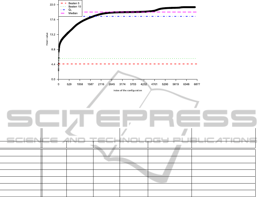
Figure 6: Sorted Set the Mean Value of all Parameterset Results.
Table 2: Comparison of the standard parameter set against the specific best parameter set;
∗
denotes the optimization with
9900 iterations, i.e., 297000 function evaluations.
Tests Reference in (Bratton and
Kennedy, 2007)
Best parameter set
Function specific specific
∗
standard gbest lbest (W,C
1
,C
2
)
Ackley 2.58 2.62 18.34 17.6628 17.5891 (0.7893,0.3647, 2.3541)
Gen. Schwefel 2154 2155 3794 3508 3360 (0.7893,2.4098, 0.3647)
Griewank 0.0135 0.0135 0.0395 0.0308 0.0009 (0.6778, 2.1142, 1.3503)
Rastrigin 6.12 6.12 169.9 140.4876 144.8155 (0.7893,2.4098, 0.3647)
Rosenbrock 0.851 0.86 4.298 8.1579 12.6648 (0.7123,1.8782, 0.5902)
Schwefel 0 0 0 0 0.1259 more than one set
Sphere 0 0 0 0 0 more than one set
4.3 Learning and Classification
As classifier we use a C4.5 decision tree. In our
implementation we use WEKA’s J4.8 implementa-
tion (Witten and Frank, 2005). As learning input we
compute 300 independent instances for each function.
Each instance consists of 32 function features. The
decision tree is created based upon the training data
and evaluated by stratified 10-fold cross-validation
(repeated 100 times). Based on the results of the ex-
tensive search we merge the classes for the objectives
Gen. Schwefel and Rastrigin into one class. These
functions share the same specific parameter set, i.e.,
the same parameter configuration performs best for
both functions. Upon these six distinct classes we
evaluate the model with cross validation. The mean
accuracy of the 100 repetitions is 84.32% with a stan-
dard deviation of 0.29. Table 3 shows the confusion
matrix of a sample classification. As it can be seen,
there are 1769 of 2100 instances classified correctly
(this means 15.76 percent of the instances are mis-
classified). The instances of the functions Ackley
and Schwefel are classified correctly with an accu-
racy of 99.7 percent, that is only one instance of these
classes is misclassified. The class for Gen. Schwefel
and Rastrigin has an accuracy of 97.2 percent. The
class Rosenbrock has a slightly lower accuracy, but
still only 5.7 percent of its members are misclassi-
fied. The high number of incorrect instances is es-
sentially due to the inability of the model to separate
the functions Sphere and Griewank. The majority of
the misclassified instances, 306 of 331, are instances
of the Griewank or Sphere class that are classified as
the other class.
4.4 Computing Effort
Computing the features is based on the evaluated fit-
ness value of specific positions in the search space.
We restrict this calculation to 3000 which means one
percent of the whole optimization process in our set-
ting. To be comparable to the benchmark of Bratton
ICAART 2011 - 3rd International Conference on Agents and Artificial Intelligence
58

Table 3: Confusion matrix of the cross validation.
classified as Accuracy Precision
class Ack. Grie. G.S./R. Rosen. Schwe. Sphe. percent percent
Ackley 299 1 99.7 99.7
Griewank 116 1 183 38.7 48.1
Gen.Schwe./Rast. 1 1 583 13 2 97.2 97.2
Rosenbrock 15 283 1 1 94.3 95.3
Schwefel 1 299 99.7 99.0
Sphere 123 1 176 58.7 48.9
and Kennedy we run the optimization for the spe-
cific parameter configuration for 9900 iterations lead-
ing to only 297000 fitness computations. We com-
pare our results of the optimization with 10000 itera-
tions to the optimization with 9900 iterations and get
quite the same results as shown in table 2 (specific vs.
specific
∗
). The comparison shows minor differences
in the magnitude of one percent.
5 DISCUSSION AND FUTURE
WORK
In this paper we describe an approach to training
a classifier which uses function features in order to
select a better parameter configuration for Particle
Swarm Optimization. We show how we compute the
features for specific functions and describe how we
get the classes of parameter sets. We include the
trained classifier and evaluate the parameter config-
uration against a Particle Swarm Optimization with
standard configuration. Our experiments demonstrate
that we are able to classify different functions on ba-
sis of a few fitness evaluations and get a parameter
set which leads the PSO to a significantly better opti-
mization performance in comparison to a standard pa-
rameter set. Statistical tests (t-Tests with α = 0.05) in-
dicate better results for the functions where the global
optimum has not been found in both settings.
The next steps are to involve all possible configu-
rations of the PSO for example the swarm size or the
neighborhood topology. These parameters are not in-
volved in our approach because we based this work
on the benchmark approach of (Bratton and Kennedy,
2007). The behavior of the swarm changes signifi-
cantly if another neighborhood is chosen. To increase
the size of the swarm is another task we will focus
in future. Depending on the swarm size different pa-
rameter sets leads to the best optimization process.
An idea is to create an abstract class of parameter
sets which include different sets of predefined swarm
sizes.
In order to get more information about the perfor-
mance of our approach it would be interesting to al-
locate a fixed percentage of the whole evaluations for
feature computation (e.g., 1%). In this case it would
be interesting to examine the quality of the result if
not all feature or features of minor quality were com-
puted.
Another extension is to define typical mathematical
function types to integrate not only one function as
class but a few functions combined under a simi-
lar type of functions to get a general set of parame-
ters. This might lead to a better generalization for the
learned classifier. The problem of this task is to find a
general problem class which defines typical kinds of
mathematical functions.
REFERENCES
Bonabeau, E., Dorigo, M., and Theraulaz, G. (1999).
Swarm Intelligence: From Natural to Artificial Sys-
tems. Oxford University Press, USA, 1 edition.
Bratton, D. and Kennedy, J. (2007). Defining a standard
for particle swarm optimization. Swarm Intelligence
Symposium, pages 120–127.
Clerc, M. and Kennedy, J. (2002). The particle swarm
- explosion, stability, and convergence in a multidi-
mensional complex space. Evolutionary Computa-
tion, IEEE Transactions on, 6(1):58–73.
Eberhart, R. and Kennedy, J. (1995). A new optimizer us-
ing part swarm theory. Proceedings of the Sixth Inter-
national Symposium on Micro Maschine and Human
Science, pages 39–43.
Hoos, H. and St
¨
utzle, T. (2004). Stochastic Local Search:
Foundations & Applications. Morgan Kaufmann Pub-
lishers Inc., San Francisco, CA, USA.
Hutter, F., Hoos, H. H., and Stutzle, T. (2007). Automatic
algorithm configuration based on local search. In Pro-
ceedings of the Twenty-Second Conference on Artifi-
cal Intelligence, (AAAI ’07), pages 1152–1157.
Kennedy, J. and Eberhart, R. (1995). Particle swarm op-
timization. Proceedings of the 1995 IEEE Interna-
tional Conference on Neural Network (Perth, Aus-
tralia), pages 1942–1948.
EXTRACTION OF FUNCTION FEATURES FOR AN AUTOMATIC CONFIGURATION OF PARTICLE SWARM
OPTIMIZATION
59

Leyton-Brown, K., Nudelman, E., and Shoham, Y. (2002).
Learning the empirical hardness of optimization prob-
lems: The case of combinatorial auctions. Principles
and Practice of Constraint Programming (CP ’02),
pages 91–100.
Pant, M., Thangaraj, R., and Singh, V. P. (2007). Parti-
cle swarm optimization using gaussian inertia weight.
In International Conference on Conference on Com-
putational Intelligence and Multimedia Applications,
volume 1, pages 97–102.
Quinlan, J. R. (1993). C4.5: Programs for Machine Learn-
ing. San Mateo, CA. Morgan Kaufmann.
Shi, Y. and Eberhart, R. C. (1998). Parameter selection in
particle swarm optimization. In Proceedings of the 7th
International Conference on Evolutionary Program-
ming VII, (EP ’98), pages 591–600, London, UK.
Springer-Verlag.
Talbi, E.-G. (2009). Metaheuristics: From design to imple-
mentation. Wiley, Hoboken, NJ.
Trelea, I. C. (2003). The particle swarm optimization algo-
rithm: convergence analysis and parameter selection.
Inf. Process. Lett., 85(6):317–325.
van den Bergh, F. and Engelbrecht, A. (2002). A new lo-
cally convergent particle swarm optimiser. Systems,
Man and Cybernetics, 2002 IEEE International Con-
ference on, 3:6 pp.
Witten, I. H. and Frank, E. (2005). Data Mining: Practi-
cal machine learning tools and techniques. Morgan
Kaufmann, San Francisco, 2nd edition.
Wolpert, D. and Macready, W. (1997). No free lunch theo-
rems for optimization. IEEE Transactions on Evolu-
tionary Computation, 1(1):67–82.
ICAART 2011 - 3rd International Conference on Agents and Artificial Intelligence
60
