
A CONTINUOS LEARNING FOR A FACE RECOGNITION
SYSTEM
Aldo F. Dragoni, Germano Vallesi and Paola Baldassarri
Department of Ingegneria Informatica, Gestionale e dell’Automazione (DIIGA)
Università Politecnica delle Marche, Via Breccebianche, Ancona, Italy
Keywords: Hybrid system, Neural networks, Bayesian conditioning, Face recognition.
Abstract: A system of Multiple Neural Networks has been proposed to solve the face recognition problem. Our idea is
that a set of expert networks specialized to recognize specific parts of face are better than a single network.
This is because a single network could no longer be able to correctly recognize the subject when some
characteristics partially change. For this purpose we assume that each network has a reliability factor
defined as the probability that the network is giving the desired output. In case of conflicts between the
outputs of the networks the reliability factor can be dynamically re-evaluated on the base of the Bayes Rule.
The new reliabilities will be used to establish who is the subject. Moreover the network disagreed with the
group and specialized to recognize the changed characteristic of the subject will be retrained and then forced
to correctly recognize the subject. Then the system is subjected to continuous learning.
1 INTRODUCTION
Several researches indicate that some complex
recognition problems cannot be effectively solved
by a single neural network but by “Multiple Neural
Networks” systems (Shields, 2008). The idea is to
decompose a large problem into a number of
subproblems and then to combine the sub-solutions
into the global one. Normally independent modules
are domain specific and have specialized
computational architectures to recognize certain
subsets of the overall task (Li, 2007). In this work,
for a face recognition problem we use a system
consisted of multiple neural networks and then we
propose a model for detecting and solving eventual
contradictions into the global outcome. Each neural
network is trained to recognize a significant region
of the face and is assigned an arbitrary a-priori
degree of reliability. This reliability factor can be
dynamically re-evaluated on basis of the Bayesian
Rule after that contradictions eventually arise. The
conflicts depend on the fact that there may be no
global agreement about the recognized subject, may
be for s/he changed some features of her/his face.
The new vector of reliability obtained through the
Bayes Rule will be used for making the final choice,
by applying the “Inclusion based” algorithm or
another “Weighted” algorithm over all the
maximally consistent subsets of the global output.
Networks that do not agree with this choice are
required to retrain themselves automatically on the
basis of the recognized subject. In this way, the
system should be able to follow the changes of the
faces of the subjects, while continuing to recognize
them even after many years thanks to this
continuous process of self training.
2 BELIEF REVISION
In this section we introduce some theoretical
background from Belief Revision (BR) field. Belief
Revision occurs when a new piece of information
inconsistent with the present belief set is added in
order to produce a new consistent belief system
(Gärdenfors, 2003).
In Figure 1, we see a Knowledge Base (KB)
which contains two pieces of information: the
information α, which comes from source V, and the
rule “If α, then not β” that comes from source T.
Unfortunately, another piece of information β,
produced by the source U, is coming, causing a
conflict in KB. To solve it we find all the
“maximally consistent subsets”, called Goods, inside
the inconsistent KB, and we choose one of them as
the most believable one. In our case (Figure 1) there
541
Dragoni A., Vallesi G. and Baldassarri P..
A CONTINUOS LEARNING FOR A FACE RECOGNITION SYSTEM.
DOI: 10.5220/0003133805410544
In Proceedings of the 3rd International Conference on Agents and Artificial Intelligence (ICAART-2011), pages 541-544
ISBN: 978-989-8425-40-9
Copyright
c
2011 SCITEPRESS (Science and Technology Publications, Lda.)
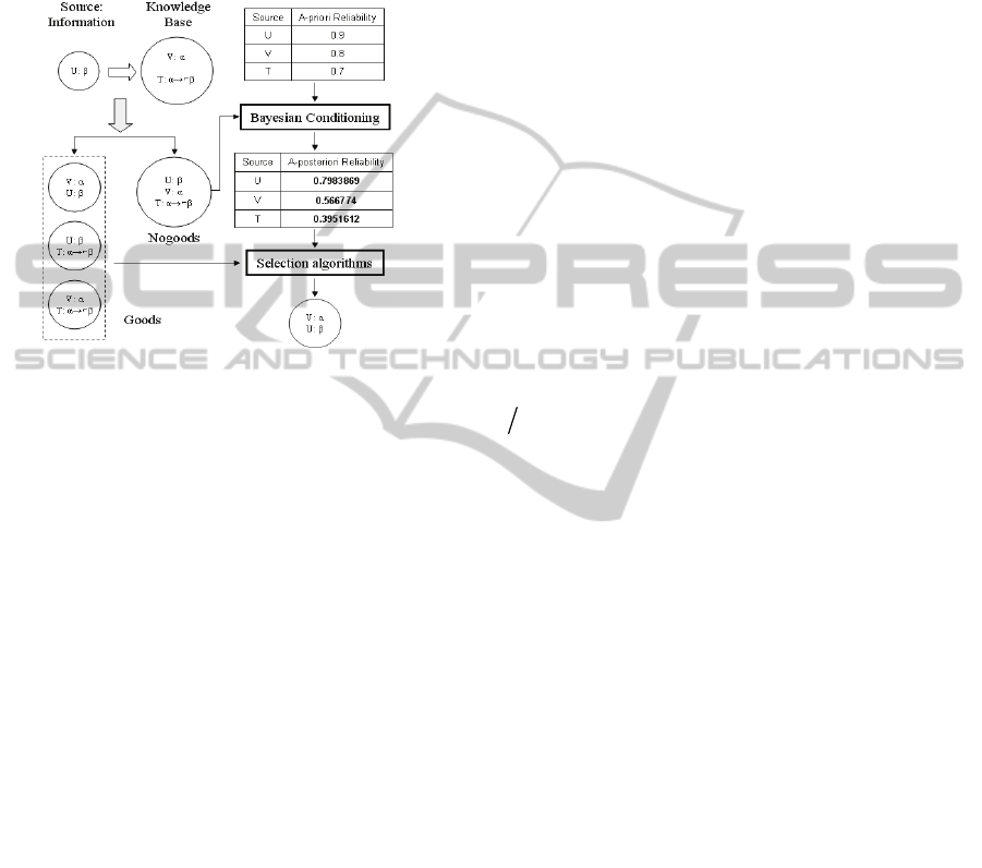
are three Goods: {α, β}; {β, α →¬β}; {α, α→¬β}.
Maximally consistent subsets (Goods) and
minimally inconsistent subsets (Nogoods) are dual
notions. Each source of information is associated
with an a-priori “degree of reliability”, which is
intended as the a-priori probability that the source
provides correct information.
Figure 1: Belief Revision mechanism.
In case of conflicts the “degree of reliability” of
the involved sources should decrease after
“Bayesian Conditioning” which is obtained as
follows. Let S = {s
1
, ..., s
n
} be the set of the sources,
each source s
i
is associated with an a-priori
reliability R(s
i
). Let
be an element of 2
S
. If the
sources are independent, the probability that only the
sources belonging to the subset
S are reliable
is:
() ( )* (1 ( ))
ss
ii
ii
R
Rs Rs
(1)
This combined reliability can be calculated for any
providing that:
2
() 1
S
R
(2)
Of course, if the sources belonging to a certain
give incompatible information, then R(
) must be
zero. Having already found all the Nogoods, what
we have to do is:
Summing up into R
Contradictory
the a-priori reliability
Putting at zero the reliabilities of all the
contradictory sets, which are the Nogoods and their
supersets
Dividing the reliability of all the other (no-
contradictory) set of sources by 1 − R
Contradictory
.
The last step assures that the constrain (2) is still
satisfied and it is well known as “Bayesian
Conditioning”. The revised reliability NR(s
i
) of a
source s
i
is the sum of the reliabilities of the
elements of 2
S
that contain s
i
. If a source has been
involved in some contradictions, then NR(s
i
) ≤ R(s
i
),
otherwise NR(s
i
) = R(s
i
).
The new “degrees of reliability” will be used for
choosing the most credible Goods as the one
suggested by “the most reliable sources”. There are
three algorithms to perform this task
1. Inclusion based (IB) Algorithm select all the
Goods which contains information provided by the
most reliable source.
2. Inclusion based weighted (IBW) is a variation of
IB: each Good is associated with a weight derived
from the sum of Euclidean distances between the
neurons of the networks. If IB select more than one
Good, then IBW selects as winner the Good with a
lower weight.
3. Weighted algorithm (WA) combines the a-
posteriori reliability of each network with the order
of the answers provided. Each answer has a weight
1n where
n1;N represents its position among
the N responses.
3 FACE RECOGNITION SYSTEM
To solve the face recognition problem (Tolba, 2006),
in the present work a number of independent
recognition modules, such as neural networks, are
specialized to respond to individual template of the
face. We apply the Belief Revision method to the
problem of recognizing faces by means of a
“Multiple Neural Networks” system. We use four
neural nets specialized to perform a specific task:
eyes (E), nose (N), mouth (M) and, finally, hair (H)
recognition. Their outputs are the recognized
subjects, and conflicts are simple disagreements
regarding the subject recognized. As an example,
let’s suppose that during the testing phase, the
system has to recognize the face of four persons:
Andrea (A), Franco (F), Lucia (L) and Paolo (P),
and that, after the testing phase, the outputs of the
networks are as follows: E gives as output “A or F”,
N gives “A or P”, M gives “L or P” and H gives “L
or A”, so the 4 networks do not globally agree.
Starting from an undifferentiated a-priori reliability
factor of 0.9, and applying the method described in
the previous section we get the following new
degrees of reliability for each network: NR(E) =
ICAART 2011 - 3rd International Conference on Agents and Artificial Intelligence
542

0.7684, NR(N) = 0.8375, NR(M) = 0.1459 and
NR(H)=0.8375. The networks N and H have the
same reliability, and by applying a selection
algorithm it turns out that the most credible Goods is
{E,N,H}, which corresponds to Andrea. So Andrea
is the response of the system.
Figure 2: Schematic representation of the Face
Recognition.
Figure 2 shows a schematic representation of this
Face Recognition System (FRS). Which is able to
recognize the most probable individual even in
presence of serious conflicts among the outputs of
the various nets.
4 A NEVER-ENDING LEARNING
Back to the example in Section III, let’s suppose that
the network M is not able to recognize Andrea from
is mouth. There can be two reasons for the fault of
M: either the task of recognizing any mouth is
objectively harder, or Andrea could have recently
changed the shape of his mouth (perhaps because of
the grown of a goatee or moustaches). The second
case is interesting because it shows how our FRS
could be useful for coping with dynamic changes in
the features of the subjects. In such a dynamic
environment, where the input pattern partially
changes, some neural networks could no longer be
able to recognize them. So, we force each faulting
network to re-train itself on the basis of the
recognition made by the overall group. On the basis
of the a-posteriori reliability and of the Goods, our
idea is to automatically re-train the networks that did
not agree with the others, in order to “correctly”
recognize the changed face. Each iteration of the
cycle applies Bayesian conditioning to the a-priori
“degrees of reliability” producing an a-posteriori
vector of reliability. To take into account the history
of the responses that came from each network, we
maintain an “average vectors of reliability”
produced at each recognition, always starting from
the a-priori degrees of reliability. This average
vector will be given as input to the two algorithms,
IBW and WA, instead of the a-posteriori vector of
reliability produced in the current recognition. In
other words, the difference with respect to the BR
mechanism described in Section II is that we do not
give an a-posteriori vector of reliability to the two
algorithms (IBW and WA), but the average vector of
reliability calculated since the FRS started to work
with that set of subjects to recognize. With this
feedback, our FRS performs a continuous learning
phase adapting itself to partial continuous changes of
the individuals in the population to be recognized.
5 EXPERIMENTAL RESULTS
This section shows only partial results: those
obtained without the feedback, discussed in the
previous section. In this work we compared two
groups of neural networks: the first consisting of
four networks and the second with five (the
additional network is obtained by separating the eyes
in two distinctive networks). All the networks are
LVQ 2.1, a variation of Kohonen’s LVQ (Kohonen,
1995), each one specialized to respond to individual
template of the face.
The Training Set is composed of 20 subjects
(taken from FERET database (Philips, 1998)), for
each one 4 pictures were taken for a total of 80.
Networks were trained, during the learning phase,
with three different epochs: 3000, 4000 and 5000.
To find Goods and Nogoods, from the networks
responses we use two methods:
1. Static method: the cardinality of the response
provided by each net is fixed a priori. We choose
values from 1 to 5, 1 meaning the most probable
individual, while 5 meaning the most five probable
subjects
2. Dynamic method: the cardinality of the response
provided by each net changes dynamically according
to the minimum number of “desired” Goods to be
searched among. In other words, we set the number
of desired Goods and reduce the cardinality of the
response (from 5 down to 1) till we eventually reach
that number (of course, if all the nets agree in their
first name there will be only one Goods).
In the next step we applied the Bayesian
conditioning (Dragoni, 1997), on the Nogoods
obtained with the two previous techniques, obtaining
an a-posteriori vector of reliability. These new
“degrees of reliability” will be used for choosing the
most credible Good (i.e. the name of subject). To
test our work, we have taken 488 different images of
the 20 subjects and with these images we have
created two Test Set. Figure 3 reports the rate of
correct recognition for the two Test Set, with the
Static and Dynamic methods. It shows also, how
WA is better than IBW for all four cases in both
A CONTINUOS LEARNING FOR A FACE RECOGNITION SYSTEM
543
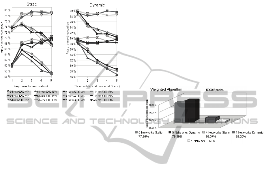
tests. The best solution for WA is achieved with five
neural networks and 5000 epochs in both the
methods (Static and Dynamic) and the Test Set.
Figure 3: Rate of correct recognition with either Test Set.
Figure 4 shows the average values of correct
recognition in either Test Set of WA with 5000
epochs obtained by the two methods. These results
show how the union of the Dynamic method with
the WA and five neural networks gives the best
solution to reach a 79.39% correct recognition rate
of the subjects. The same Figure also shows as using
only one LVQ network for the entire face, we obtain
the worst result. In other words, if we consider a
single neural network to recognize the face, rather
one for the nose and so on, we have the lowest rate
of recognition equals to 66%. This is because a
single change in one part of the face makes the
whole image not recognizable to a single network,
unlike the hybrid system.
6 CONCLUSIONS
Our hybrid method integrates multiple neural
networks with a symbolic approach to Belief
Revision to deal with pattern recognition problems
that require the cooperation of multiple neural
networks specialized on different topics. We tested
this hybrid method with a face recognition problem,
training each net on a specific region of the face:
eyes, nose, mouth, and hair. Every output unit is
associated with one of the persons to be recognized.
Each net gives the same number of outputs. We
consider a constrained environment in which the
image of the face is always frontal, lighting
conditions, scaling and rotation of the face being the
same. We accommodated the test so that changes of
the faces are partial, for example the mouth and hair
do not change simultaneously, but one at a time.
Under this assumption of limited changes, our
hybrid system ensures great robustness to the
recognition. When the subject partially changes its
appearance, the network responsible for the
recognition of the modified region comes into
conflict with other networks and its degree of
reliability will suffer a sharp decrease. The networks
that do not agree with the choice made by the overall
group will be forced to re-train themselves on the
basis of the global output. So, the overall system is
engaged in a never ending loop of testing and re-
training that makes it able to cope with dynamic
partial changes in the features of the subjects.
Figure 4: Average rate of correct recognition with either
Test Set and the results obtained using only one network
for the entire face.
REFERENCES
Shields, M. W., Casey, M. C., 2008. A theoretical
framework for multiple neural network systems.
Neurocomputing, vol. 71, pp. 1462–1476.
Li, Y., Zhang, D., 2007. Modular neural networks and
their applications in biometrics. Trends in Neural
Computation, vol. 35, pp. 337–365.
Gärdenfors, P., 2003. Belief Revision, Cambridge Tracts
in Theoretical Computer Science, vol. 29.
Tolba, A. S., El-Baz, A. H., El-Harby, A. A., 2006. Face
recognition a literature review, International Journal
of Signal Processing, vol. 2, pp. 88–103.
Kohonen, T., 1995. Learning vector quantization, in Self-
Organising Maps, Springer Series in Information
Sciences. Berlin, Heidelberg, New York: Springer-
Verlag, 3rd ed.
Philips, P. J., Wechsler, H., Huang, J. Rauss, P., 1998. The
FERET Database and Evaluation Procedure for Face-
Recognition Algorithms. Image and Vision Computing
J., vol. 16, no. 5, pp: 295-306.
Dragoni, A. F., 1997. Belief revision: from theory to
practice. The Knowledge Engineering Review, vol. 12,
no. 2, pp:147-179.
ICAART 2011 - 3rd International Conference on Agents and Artificial Intelligence
544
