
MORPHOLOGICAL ANALYSIS OF 3D PROTEINS STRUCTURE
Virginio Cantoni, Riccardo Gatti and Luca Lombardi
University of Pavia, Dept. of Computer Engineering and Systems Science, Via Ferrata 1, Pavia, Italy
Keywords: Structural biology, Protein structure analysis, Protein-ligand interaction, Surface segmentation.
Abstract: The study of the 3D structure of proteins supports the investigation of their functions and represents an
initial step towards protein based drug design. The goal of this paper is to define a technique, based on the
geometrical and topological structure of protein surfaces, for the detection and the analysis of sites of
possible protein-protein and protein-ligand interactions. In particular, the aims is to identify concave and
convex regions which constitute ‘pockets’ and ‘protuberance’ that can make up the interactions ‘active
sites’. A segmentation process is applied to the solvent-excluded-surface (SES) through a sequence of
propagation steps applied to the region between the protein convex-hull and the SES: the first phase
generates the pockets (and tunnels) set, meanwhile the second (backwards) produces the protrusions set.
1 INTRODUCTION
In the last decade much work has been done on the
detection and analysis of binding sites of proteins
through bioinformatics tools. This is a preliminary,
but important step that can reduced consistently the
cost, in time and resources, of the subsequent
experimental validation phase, which is applied only
to the resulting subset loci. It is worth to point out
that the effective identification of active sites is
instrumental for structure-based drug development
and design.
The various approaches proposed up-to-now are
characterized by the solution of two subproblems:
the protein representation and the matching
strategies. Among the techniques that have been
proposed up to now, we can quote: the geometric
hashing of triangles of points on the SES and their
associated physico-chemical properties (Laskowski,
1995); a representation of the SES in terms of
spherical harmonic coefficients (Glaser, 2006); a
collection of spin-images (Glaser, 2006) (Bock,
2007); a ‘context shapes’ representation (Binkowski,
2003); a set of vertices of the triangulated solvent-
accessible surface (SAS) (Shulman, 2004).
Recently, a few packages for the process of
detecting and characterizing candidate active sites
are supplied on the web. The most known packages,
in chronological sequence, are here shortly
described.
The first POCKET (Levitt, 1992) has been
developed in the early ‘90. The protein is mapped
onto a 3D grid, and a grid point belongs to the
protein if it is within 3 Å from an atom nucleus. The
pockets consist of the set of grid points, in the
solvent area for which a scanning along the x, y, or
z-axes presents a sequence protein-solvent-protein.
More recently LIGSITE (Huang, 2006) extends
POCKET by scanning also along the four cubic
diagonals (in fact, the POCKET’s classification is
dependent on the angle between the reference
system and the protein). The solvent points that
present a number of protein-solvent-protein events
greater than a given threshold are classified as
candidate active sites.
In the late ’90 CAST (Liang, 1998) (updated
with CASTp (Binkowski, 2003) in the early ’00),
based on 3D computational geometry, has been
proposed. In this approach the protein is represented
by a set of 3D tetrahedra having the vertices on the
nucleus positions and is analyzed through convex-
hull, alpha shapes and discrete flow theory. A
tetrahedron having at least a facet crossing the
solvent region is designated as ‘empty tetrahedron’.
Empty tetrahedra sharing a common triangle are
grouped so ‘flowing’ towards neighbouring larger
tetrahedra which act as sink. A pocket, which is a
potential binding site, is a collection of empty
tetrahedra. Pockets volume, mouth opening area and
circumference are easily evaluated on this structure.
15
Cantoni V., Gatti R. and Lombardi L..
MORPHOLOGICAL ANALYSIS OF 3D PROTEINS STRUCTURE.
DOI: 10.5220/0003127000150021
In Proceedings of the International Conference on Bioinformatics Models, Methods and Algorithms (BIOINFORMATICS-2011), pages 15-21
ISBN: 978-989-8425-36-2
Copyright
c
2011 SCITEPRESS (Science and Technology Publications, Lda.)

PASS (Brady, 2000), introduced in the early ’00,
is based on a purely geometrical method consisting
in a sequence of steps: i) the protein surface, on the
side of the solvent, is completely covered by probe
spheres each one not contained in any others; ii)
each probe is associated with a “burial” value, which
corresponds to the number of atoms contained
within a concentric sphere of radius 8 Å; iii) the
probes with a “burial” value lower than a predefined
threshold are eliminated; iv) the previous three steps
are iterated (with step one applied only to surface’s
patches covered by the probes) until the regime,
where no new buried probe can be added; v) a probe
weight, which is dependent on the number of the
neighbouring spheres and the extent to which they
are buried, is assigned; vi) a shortlist of active site
points (ASPs), ranked by the probe weight, is
identified through the central probes that contain
many spheres with high burial count.
Finally SURFNET-ConSurf (Glaser, 2006) is
based on a pocket-surface representation which
combines geometrical features together with an
evolutionary parameter based on the degree of
conservation of the amino acids involved. Initially,
through SURFNET (Laskowski, 1995), the clefts are
detected by placing a sphere between all pairs of
atoms such that the sphere just touches each atom of
the pair, then this sphere is progressively reduced in
size up to no further intersections with other atoms
are present. The resulting sphere is retained only if
its radius is greater than a minimum size predefined.
Moreover, the regions that do not present highly
conserved residues, as defined by the ConSurf-HSSP
database (Glaser, 2005), are removed, thus reshaping
the cleft volumes. The remaining clefts are candidate
active sites (in particular the largest ones).
In this paper we present a new method for two
segmentations of the SES with the aim of identifying
respectively the concavities that can host a ligand or
a protrusion of another protein and the protuberances
that can match the inlet of others proteins. The paper
is organized as follows: in section two we describe a
new technique that, starting from the protein
enlarged convex hull, propagates up to the SES to
identify concave active sites; in section three a
second backward propagation algorithm that detect
the protuberances, starting from the peaks of the
previous propagation is introduced. In section four a
few practical cases and some comparisons are given.
Section five contains the conclusion and our near
future subsequent activities.
2 LOOKING FOR POCKETS AND
TUNNELS
The first half of this procedure has been already
introduced in (Cantoni, 10a). This segmentation is
based on a propagation process (a Distance
Transform (DT)) applied to the volume obtained
subtracting the molecule to its Convex Hull (CH).
Before presenting this process, here a few
preliminary definitions and statements are given.
The CH of a molecule is the smallest convex
polyhedron that contains the molecule points. In R
3
the CH is constituted by a set of facets, that are
triangles, and a set of ridges (boundary elements)
that are edges. A practical O(n log n) algorithm for
general dimensions CH computing is Quickhull
(Barber, 1996), that uses less memory space and
executes faster than most of the other algorithms.
The protein and the CH are defined in a cubic
grid V of dimension L x M x N voxels. Note that the
grid is extended one voxel beyond the minimum and
maximum coordinate of the SES in each orthogonal
direction (in this way both SES and CH borders are
always inside the V border). The voxel resolution
adopted is 0.25 Å, so as to be small enough to ensure
that, with the used radii in biomolecules atoms, any
concave depression or convex protrusion is
represented by at least one voxel.
Let us call R the region between the CH and the
SES (the concavity volume (Borgefors, 1996), that
is:
R= CH∩SES
(1)
Let us call B
CH
the set of the border voxels of
CH, that is:
B
=CH−[CH∎K]
(2)
where ∎ represent the erosion operator of
mathematical morphology (Serra, 82) and K the
discrete unitarian sphere (in the discrete space, in 26
connectivity, a 3x3x3 cube!). Within the region R
the following propagation is applied:
D
=
1iϵB
0ℎ
A = B
CH
;
N = (A ⊕ K)∩R;
E = N – A;
while E ≠ ∅ do
∀e ∈ E:
= min
∈
(
+
)
A = N;
N = (A ⊕ K)∩R;
E = N – A;
done
BIOINFORMATICS 2011 - International Conference on Bioinformatics Models, Methods and Algorithms
16

where:
i.
A represents the increasing set of voxels
contained in R; E corresponds to the recruited
set of near neighbors of A contained in R (i.e.
the voxels reached by the last propagation step);
ii. min
∈
(
+
)
represents the minimum
value among the distances
in the near
neighbors belonging to D already defined,
incremented by the displacement
between
the locations (e, n): that is, if e and n have a
common face
=1; if e and n have a
common edge
=
√
2; if e and n have a
common vertex
=
√
3. In three dimensions,
the total number of the near neighbor elements
of p is 26: six of them that share one face and
have distance equal to 1 from the voxel p,
twelve neighbors that share only an edge and
are at distance
√
2
, and eight that share only a
vertex and are at distance
√
3
always from voxel
p. At each iteration, new voxels, inside R, are
reached by the propagation process and the
value they take is determined by the minimum
of the neighbor distances (from the CH)
increased by the relative voxels distance; this in
order to simulate an isotropic propagation
process and the digital distance evaluation.
iii. E = ∅ corresponds to the regime condition: no
other changes are given and the connected
component of R, adjacent to the border B
CH
,
is
completely covered.
The values in D represent the distance of each
voxel of A from B
CH
and A corresponds to the
connected component of R adjacent to the border.
Having A, it is possible to easily identify and
eventually remove the cavities C, that are the
volumes completely enclosed in the macromolecule
M:
C = CH - A - M
(3)
In order to identify the different pockets and
tunnels the volume A must be partitioned into a set
of disjoint segments P
SES
={P
1
, … , P
j
, … , P
N
},
where N is the number of inlets. The partition must
satisfy the following condition:
P
i
∩ P
j
= ∅, i ≠ j
(4)
P
1
∪ ·· · ∪ P
j
∪ ·· · ∪ P
N
= A
(5)
As can be easily realized, starting from the total
set of convex hull facets, several waves are
generated and propagation proceeds up to the
complete coverage of the volume A: the connected
component of R adjacent to the border. During the
propagation phase two sets of salient points are
identified: local tops LT and wave convergence WC
points.
The LT set is exploited for the segmentation
process. The cardinality of LT corresponds to N
max
the maximum number of segments/inlets that can be
considered. The effective number of segments, that
determines obviously the number and the
morphology of pockets and tunnels, is found out on
the basis of two heuristic parameters: i) the
minimum travel depth value of the local tops TD
LT
;
ii) an evaluation of the near tops pivoting effects
PEs. The threshold TD
LT
is introduced because the
surface’s irregularities and the digitalization process
produce small irrelevant spurious cavities. Two
thresholds are introduced on the basis of PEs taking
into account morphological aspects insight important
cavities: the nearness of others, more significant,
local tops (τ
1
) and the relative values of the local-top
travel-distance (τ
2
). A detailed description of this
first phase is given in (Cantoni, 10a).
The second phase is completely new. Let us
assume that a pocket has at least the volume of a
water molecule. Under this assumption we will
identify the useful portion of A by:
B=A∎S
(6)
Where ∎ represent the erosion operator and S
the minimum sphere that contains a water molecule.
The set of voxel E
A
given in (7) constitutes the fine
grains with a too strong concavity (figure 2):
E
=A−B
(7)
Figure 1: SES of PDB ID 1MK5 and its extended CH.
The results achieved in this phase are shown in
figure 1. In general, the set LT is contained in the set
EA. Using as seed-points the set LT, a back-
propagation toward Bch is performed. At each step
the new connected voxels having the same distance
(de) are joined to the seed set ST. A candidate
MORPHOLOGICAL ANALYSIS OF 3D PROTEINS STRUCTURE
17
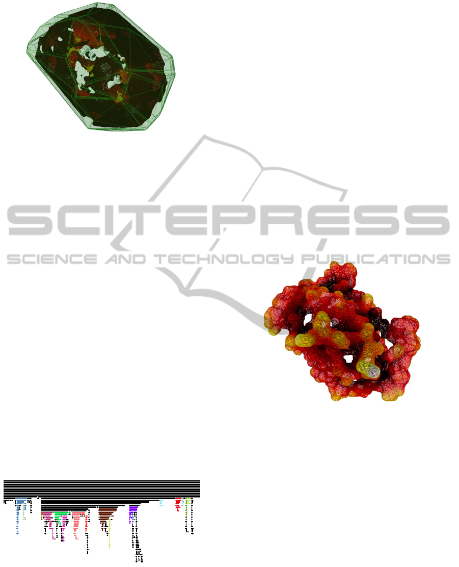
Figure 2: the set E
a
of PDB ID 1MK5.
pocket is established active when ST maintains at
each step at least a new voxel belonging to B.
During the propagation towards Bch , if the new
joined set of voxels is completely contained in EA a
bottleneck has been reached and the seed set ST in
progress is anymore active.
i) When two or more seed sets converge there are
three possible cases: all the convergent sets are
active: in this case a new active set is generated
on the basis of the union of the new entry
voxels;
ii) among the convergent sets there is at least one
active set: this set continues the propagation (if
there is more than one active set it is first
applied the case i) recursively) including the
convergent new entry voxels of the connected
not active set(s);
iii) all the convergent sets are not active: this
means that some fine grains are joining
together, and a new propagation seed
composed by the union of the entry voxels is
established if this union achieves a volume at
least equal to the water molecule.
In figure 3 it is shown for the protein 1MK5 a 2D
sketch representing the final result of this process.
Figure 3: A portion of the 2D sketch achieved by applying
the pocket search algorithm on the protein 1MK5. The
vertical clusters that are not associated to any pockets are
black, meanwhile the ones representing pockets are
colored.
3 LOOKING FOR
PROTUBERANCES
The objective here is to segment the SES to
underline the protuberances. There is a duality
relationship between this process and the previous
one: pockets are SES segments mainly concave,
meanwhile protuberances are mainly convex. Let us
assume that protuberances we are looking for have a
known maximum section area contained in a circle
of radius r. Under this assumption we will identify a
basis volume F by:
F = SES ■ S
r
(8)
where ■ represents the erosion operator (Serra,
1982) and S
the sphere of radius r.
Let us call S
F
the external surface of F. The set of
voxel G given in (9) constitutes the working volume
(figure 4) for our analysis by:
G = SES - F
(9)
Figure 4: volume G for PDB ID 1MK5 for a sphere Sr of
radius 2.4 Å.
Within the region G in a similar way of the previous
pocket search, the following propagation is applied:
D
=
1iϵS
F
0ℎ
N = (A ⊕ K)∩G;
E = N – A;
while E ≠ ∅ do
∀e ∈ E:
= min
∈
(
+
)
A = N;
N = (A ⊕ K)∩G;
E = N – A;
Done
where: A represents the increasing set of voxels
contained in G; E corresponds to the recruited set of
near neighbors of A contained in G (i.e. the voxels
BIOINFORMATICS 2011 - International Conference on Bioinformatics Models, Methods and Algorithms
18
reached by the last propagation step); the values in D
represent the distance of each voxel of A from S
.
Starting from the S
′s voxels (to which a
common label is assigned), a new recursive scanning
phase within G is applied, going toward SES. At
each step, the new entry voxels are segmented in
connected sets. When there is a one-to-one
correspondence between a new segment set and a set
of the previous step, its label is extended to the new
segment. When a previous set is split in two or more
segment sets a new label is generated for each one of
them.
As in the propagation process for the search of
pockets, during the propagation phase, two sets of
salient points are identified: local tops LT and wave
convergence WC points. Both these salient points
are important for the docking analysis. A 2D sketch
representing the final result is shown in figure 5.
Figure 5: A portion of the 2D sketch achieved by applying
the protuberances search algorithm on the protein 1MK5.
The vertical clusters that are not associated to any pockets
are black, meanwhile the ones representing pockets are
colored. Note that different vertical clusters have the same
color when they are joined to the same protuberance.
4 EXPERIMENTS
AND COMPARISONS
As an example, the proposed technique has been
applied to the Apostreptavidin Wildtype Core-
Streptavidin with Biotin structure (PDB ID: 1MK5).
The analysis has been done with a resolution of 0.25
A°, which entails a van der Waals radius of more
than five voxels to the smallest represented atoms.
The SES is obtained from the van der Waals surface,
after the execution of a closure operator, using a
sphere with radius of 1.4 A°, approximately 6 voxels
(corresponding to the conventional size of a water
molecule), as structural element.
For what concerns the pockets detection the three
parameters have been set as follows: the minimum
travel depth of the local tops to TD
LT
= 5 voxels; the
nearness of others, more significant, local tops to τ
1
=
150 voxels and the relative values of the local-top
travel-distance to τ
2
= 2000 voxels. Moreover, the
radius of the water molecule has been set to 6
voxels.
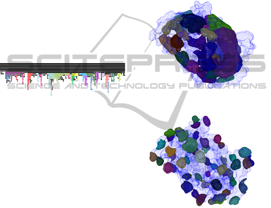
In figure 6 it is shown the final result of the
segmentation process of the protein 1MK5 for the
detection of pockets and tunnels. Note that among
the 25 pockets that have been detected, 2 have a
volume greater than 80 water molecules and have a
travel depth of 26 voxels and mouth aperture of
8.343 and 30.547 respectively.
Figure 6: Final result of the segmentation process of PDB
ID 1MK5 for the detection of pockets.
Figure 7: Final result of the segmentation process of PDB
ID 1MK5 for the detection of protuberances.
Figure 7 shows the final result of the
segmentation process of the protein 1MK5 for the
detection of protuberances. The parameter r
representing the maximum section area has been set
to 800 voxels. Note that among the 41 protuberances
that have been detected 9 have a volume greater than
7 water molecules, and a base aperture of 22.968,
8.236, 16.000, 9.287, 8.444, 9.008, 7.469, 11.148,
9.684 voxels respectively.
All the packages quoted in this paper’s
introduction are related to just pockets and tunnels
MORPHOLOGICAL ANALYSIS OF 3D PROTEINS STRUCTURE
19

detection, at the authors knowledge there are not
packages specialized for segmenting the SES on the
basis of protuberances. Among the quoted packages
the only one that was available and directly
applicable has been CASTp. We compared the
results obtained with this package to our one. The
number of pocket selected has been 29 and 25
respectively for CASTp and our own. Let us first
point out that all the main pockets of the quoted
protein (the bigger and deeper ones) are detected in
both cases. Moreover, for the main pockets, almost
the same set atoms at the border of the SES
delimiting the pockets. Nevertheless, in general the
number of these atoms is higher in our solution (up
to 20% in a few cases) and seems to cover in a
complete way the pocket concavity. An example of
this case is given in figure 8.
Figure 8: Wireframe of the main binding site of PDB ID
1MK5. In red atoms detected by CASTp. Our software
detects both the red and green atoms.
The results differ more for what concerns the
smallest pockets. This is due to the thresholds to
accept the concavity with a short travel depth as a
possible active site. We have two thresholds on the
basis of the travel depth and of a minimum
concavity volume. Generally speaking CASTp
accept more small concavities as pockets, but
sometimes there are cases in which our volume
constraint is satisfied and the concavity is not
accepted by CASTp. This must not be a critical
issues because (Liang, 1998) the binding sites are
usually the pockets having the greatest volume.
While CASTp includes empty volume internal to the
protein, in our approach these are identified but not
classified as pockets.
Referring to computational performance, our
algorithm runs on an Intel Q6600 Processor with 4
GB of Ram. The analysis of pockets and
protuberances on 1MK5 protein as been done in 58
seconds starting from the PDB file (this include the
operations of creating the 3D matrix, the Convex
Hull, all mathematical morphology operations, the
triangulation of the voxels surface of each
pocket/protuberance with a marching cube/mesh
smoothing algorithm and so on). In fact besides the
segmentation process for each detected segment
(pocket or protuberance) a rich parameter set is
computed to guide the analysis of possible match,
such as volume, surface to volume ratio, mouth
(base) aperture, travel depth, and many others (a full
list is given in (Cantoni, 10b). It is important to note
that all the algorithms presented in this paper are
already thought to be simply implemented into
parallel architectures.
5 CONCLUSIONS
In this paper we present a new approach for the
segmentation of SES of proteins in order to support
the search of dual active sites (i.e. pockets and
protuberances) that can be morphologically arranged
together. This is a preliminary step for important
structural biology application. The results achieved
look very promising and in comparison to others
solutions presented in literature it seems to add
something not only from the computational point of
view. Now we have started an extensive
experimentation phase to validate our solution from
the best practice point of view.
REFERENCES
Barber, C. B., Dobkin, D. P., and Huhdanpaa H., 1996.
The Quickhull Algorithm for Convex Hull. ACM
Transactions on Mathematical Software, Vol. 22(4):
469–483.
Binkowski, A. T., Naghibzadeh, S., and Liang, J., 2003.
Castp: Computed atlas of surface topography of
proteins. Nucl. Acids Res.,31(13): 3352- 3355.
Bock, M. E., Garutti C., Guerra C., 2007. Effective
labeling of molecular surface points for cavity
detection and location of putative binding sites. Proc.
of CSB, San Diego, Vol. 6: 263-744.
Borgefors, G. and Sanniti di Baja, G., 1996. Analyzing
Nonconvex 2D and 3D Patterns. Computer Vision and
image Understanding, 63(1): 145– 157.
Brady, G. P., Stouten, P. F. W., 2000. Fast prediction and
visualization of protein binding pockets with PASS. J
Comput-Aided Mol Des, 14: 383–401.
Cantoni, V., Gatti, R., Lombardi, L., 2010. Segmentation
of SES for Protein Structure Analysis. In Proceedings
of the 1st International Conference on Bioinformatics.
BIOINFORMATICS 2011 - International Conference on Bioinformatics Models, Methods and Algorithms
20

BIOSTEC 2010: 83–89 (a).
Cantoni, V., Gatti, R., Lombardi, L., 2010. Proteins
Pockets Analysis and Description. In Proceedings of
the 1st International Conference on Bioinformatics.
BIOSTEC 2010: 211–216 (b).
Glaser, F., Rosenberg, Y., Kessel, A., Pupko, T. and
Bental, N., 2005. The consurf-hssp database: the
mapping of evolutionary conservation among
homologs onto pdb structures. Proteins, 58(3): 610-
617.
Glaser, F., Morris, R. J., Najmanovich, R. J., Laskowski,
R. A. and Thornton, J. M., 2006. A Method for
Localizing Ligand Binding Pockets in Protein
Structures. PROTEINS: Structure, Function, and
Bioinformatics, 62: 479-488.
Huang, B., Schroeder, M., 2006. LIGSITEcsc: predicting
ligand binding sites using the Connolly surface and
degree of conservation. BMC Structural Biology, 6:19.
Laskowski, R. A., 1995. Surfnet: a program for visualizing
molecular surfaces, cavities and intermolecular
interactions. J Mol Graph, 13(5), 323-30.
Levitt, D. G. and Banaszak, L. J., 1992. Pocket: a
computer graphics method for identifying and
displaying protein cavities and their surrounding
amino acids. J Mol Graph, 10(4): 229–234.
Liang, J., Edelsbrunner, H. and Woodward, C., 1998.
Anatomy of protein pockets and cavities: measurement
of binding site geometry and implications for ligand
design. Protein Sci, 7(9): 1884- 1897.
Serra, J., 1982. Image analysis and mathematical
morphology. Academic Press.
Shulman-Peleg, A., Nussinov, R. and Wolfson, H., 2004.
Recognition of Functional Sites in Protein Structures.
J. Mol. Biol., 339: 607–633.
MORPHOLOGICAL ANALYSIS OF 3D PROTEINS STRUCTURE
21
