OPTIMAL CONTROL OF MIXED-STATE QUANTUM
SYSTEMS BASED ON LYAPUNOV METHOD
Shuang Cong, Yuanyuan Zhang
Department of Automation, University of Science and Technology of China, Hefei, Anhui, 230027, Republic of China
Kezhi Li
Dept.of Electrical and Electronic Engineering, Imperial College London, South Kensington Campus
London SW7 2AZ, U.K.
Keywords: Optimal control, Lyapunov-based control, Quantum systems, Mixed state, Oscillator.
Abstract: An optimal control strategy of mixed state steering in finite-dimensional closed quantum systems is
proposed in this paper. Two different situations are considered: one is the target state is in statistical
incoherent mixtures of energy eigenstates in which the target states are diagonal. Another is not all of the
off-diagonal elements in the target states are zeros. We change the trajectory tracking problem into the state
steering one by introducing the unitary transformation with all energy eigenstates in the inner Hamiltonian
of system controlled. Based on Lyapunov stability theorem the stable parameters of controller designed is
selected and the optimality of the control law proposed is proven. Moreover, two numerical system control
simulations are performed on the diatomic molecule described by the Morse oscillator model under the
control law proposed. The system control simulation experimental results demonstrate that the control
strategies proposed are efficient even when the controlled system is not completely controllable
.
1 INTRODUCTION
As one of the greatest achievements in the 20th
century, quantum mechanics has urged the human
view of the matter to the microcosm. An enormous
amount of revolution in theory and engineering
science have been undertaken due to the
development and applications of quantum physics,
quantum chemistry, quantum computation and
quantum information. (Nielsen and Chuang, 2000).
In these new interdisciplinary fields, how to control
the quantum systems has become a challenging
subject. One part of the quantum control theories is
about the applications of classical and modern
control theory to quantum systems. (
Wang and
Schirmer, 2008) Now there have been various control
schemes applied to the quantum systems, such as the
Lyapunov-based method (Grivopoulos and Bamieh,
2003; Mirrahimi, Rouchon, and Turinici, 2005;
Beauchard et al. 2007; Cong and Kuang, 2007;
Kuang and Cong, 2008), optimal control method
(Peirce, et al. 1988; D’Alessandro and Dahleh,
2001; Girardeau, et al. 1998; Schirmer, et al. 2000),
learning control method (
Judson and Rabitz, 1992;
Phan and Rabitz, 1999), state estimation method
(
Doherty and Jacobs, 1999; Zhang, Li, and Guo, 2000),
and stochastic control method (Belavkin, 1992;
Bouten, et al. 2004), etc. Generally, the control aim
of a quantum system is to search for a control field
by means of minimizing an energy-type cost
function of system that usually requires a maximal
transition probability from an initial state to a
particular target state. Among all of the quantum
control strategies, optimal control methods are the
most popular approaches that have been widely used
specially in quantum chemistry fields. Since the mid
1980s, the quantum optimal control theory has
attracted attentions from many researchers.
However, many proposed optimal control methods
are generally obtained by means of complex numeral
iterative algorithms, which are off-line control
methods and quite inconvenient to operate and
realize. Thus, how to obtain an optimal method
without iterative solutions is of great significance.
22
Zhang Y., Cong S. and Li K..
OPTIMAL CONTROL OF MIXED-STATE QUANTUM SYSTEMS BASED ON LYAPUNOV METHOD.
DOI: 10.5220/0003126000220030
In Proceedings of the International Conference on Bio-inspired Systems and Signal Processing (BIOSIGNALS-2011), pages 22-30
ISBN: 978-989-8425-35-5
Copyright
c
 2011 SCITEPRESS (Science and Technology Publications, Lda.)

There is another method called local optimal
control which defines a general performance index
()yt as a function of the expectation values of
physical observables. Then it designs a control field
that drives the quantum system satisfying the
monotonous increasing condition of
()yt (Ohtsuki,
1998; Sugawara, 2003). Local optimal law is
explicitly derived without iteration and can satisfy
the necessary condition for a solution to the optimal
control problem. In the applications of optimal
control theory, we can select different performance
index and get different control laws. Here we will
select the error between the states as a performance
index of the control law. The difference between
Ohtsuki (1998), Sugawara (2003) and this paper is
that the derived control law in this paper satisfies the
sufficient condition for optimal. We have applied
this method to a pure state quantum system (
Zhang
and Cong, 2008). As a further step, in this paper we
would like to consider the mixed-state control
problem based on the formulas of statistical
mechanics, and apply the idea in Ref. Zhang and
Cong (2008) to the Liouville equation. In quantum
system, two reasons lead to mixed-state: one is
quantum dissipation due to quantum system entangle
with environment. In such a situation, the system
will be open. Quantum state will become a mixed-
state even though it is a pure state at the beginning.
Here, evolution of density matrix in this open system
will not be unitary. Second, a mount of same
particles in different pure states are incoherent
mixed, which would be a quantum ensemble.
Particles in different pure states are in this ensemble
with some probability, viz. average statistically. In
this paper, we only consider closed system without
action with environment, so mixed-state here refers
to mixed-state in ensemble.
The rest of the paper is organized as follows. In
Sec. 2 we introduce the system models in Hilbert
space and in Liouville space. Section 3 gives the
control law theorem and its proof based on the
Lyapunov stability theorem and principle of
optimality under the condition that the target state is
diagonal and non-diagonal, respectively. The
numerical simulation on the diatomic molecule
described by the Morse oscillator model is presented
in Sec. 4. Finally, Sec. 5 concludes the study of the
paper.
2 MODEL OF THE SYSTEM
CONTROLLED
The state of a quantum mechanical system can be
described in various ways. When a system is in a
pure state un-entangled with its environment, the
state of the system can be described by a wave
function that evolves according to a control-
dependent Schrödinger equation. One can also
describe the state of the system by a density operator
ˆ
()t
ρ
, which can not only represent a pure state but
also a mixed state. The density operator
ˆ
()t
ρ
acting on the system’s Hilbert space H evolves
with time according to the quantum Liouville
equation:
ˆ
ˆˆ
() [ (), ()]itHtt
t
ρρ
∂
=
∂
= ,
0
1
ˆ
ˆ
ˆ
() ()
M
mm
m
H
tH ftH
=
=+
∑
(1)
where
0
ˆ
H
is the system’s internal (or free)
Hamiltonian, and
ˆ
m
H
is the interaction (or control)
Hamiltonian, respectively, all of them will be
assumed to be time-independent.
()
m
f
t is the
admissible real-valued external control field. We set
the Planck constant 1
=
= for convenience.
Because
ˆ
()t
ρ
is a NN× density matrix in
Hilbert space, it’s difficult to solve the differential
Eq. (1). One may introduce the Liouville operator in
the Liouville space according to the concept of Dirac
operator to simplify this problem. There is a natural
connection between the density matrix and Liouville
space (Barnett and Dalton, 1987; Ohtsuki, et al.
1989). In the Liouville space, Eq. (1) can be
represented in the same form as the Schrödinger
equation
() () ()it tt
t
ρρ
∂
=
∂
L ,
0
1
() ()
M
mm
m
tft
=
=+
∑
LL L
(2)
where
()t ρ is defined as a Liouville ket, and L
is the Liouville operator defined by the dual
correspondence
ˆ
ˆ
() () [ , ()]tt Ht
ρρ ↔L
(3)
The basis vectors respectively belonging to
Liouville space and Hilbert space are defined by the
OPTIMAL CONTROL OF MIXED-STATE QUANTUM SYSTEMS BASED ON LYAPUNOV METHOD
23

bijective correspondence
mn m n↔
(Schirmer, 2000). Then one has
,
*
ˆ
[, ]
ˆ
([, ])
ˆˆ
()
ˆ
ˆ
jk mn
i
nk jm jm nk kn jm
jk mn j H m n k
tr k j H m n
ik jHmni ik jmnHi
jHm nHk H H
δδδδ
==
=
=−
=−=−
∑
LL
(4)
For an NN× density matrix
ˆ
()t
ρ
in Hilbert
space, its replacement form
()t ρ is an
2
N
column vector in Liouville space, and L is an
22
NN× matrix. In such a way it is much easier to
solve Eq. (2) than Eq. (1) expressed in terms of
some commutators. Hence, Eq. (2) will be adopted
as the investigated model in following sections of
the paper.
3 CONTROL LAW DESIGN
The quantum control problems can be formulated in
state steering (or transfer) problem, that is to say
steer the system from a given initial state to a
desired target state. In this section we’ll develop an
optimal control method based on Lyapunov theorem
for the Liouville equation.
First we will introduce principle of optimality
and the sufficient condition for optimality. Suppose
the controlled system is in the form
of () [ (), (),]tttt=
xfxu

, where
12
[, ]tTT∈ ,
12
() [ , ]
n
tTT⊂×x \ ,
12
() [ , ]
m
tTT⊂×u \ . Let X be
a given region in
12
[, ]
n
TT×\ and contain the
target set
S . For each
00
(,)tx in X , one need
determine the control
u which transfers
00
(,)tx
to
S and minimizes the performance index
1
0
(, ,) [(), (),]d
t
t
J
tLtttt=
∫
xu x u . Define
*
(,)
J
tx is the
minimum of ( , , )
J
txu . The Hamiltonian
(, , ,)
H
txpu is given by
(, , ,) (, ,) ,(, ,)
H
tL t t=+〈 〉xpu xu pf xu
Principle of Optimality: If
*
()tu is an optimal
control and if
*
()tx , for
01
[,]ttt∈ , is the optimal
trajectory corresponding to
*
()tu , then the
restriction of
*
()tu to a subinterval
1
[, ]tt of
01
[,]tt is an optimal control for the initial pair
*
((),)ttx .
Sufficient Condition for Optimality (Athans and
Falb, 1966): Suppose that
12
(, )
n
XTT=×\ ,
H
is
normal relative to
12
(, )
n
TT×\ , and ( , , )tuxp is
the
H
-minimal control relative to
12
(, )
n
TT×\ .
Let
*
()tu be an admissible control such that:
a.
*
()tu transfers
00
(,)tx to S .
b. There is a solution
*
(,)
J
tx of the
Hamilton-Jacobi equation
(,) [, (,), (, (,),),] 0
JJJ
t H t ttt
t
∂∂∂
+
=
∂∂∂
xxxuxx
xx
satisfying the boundary condition ( , ) 0Jt=
x for
(,)tS
∈
x , such that
*
** *
( ) ( ( ), ( ( ), ), )
J
tt ttt
∂
=
∂
ux x
x
for t in
01
(,)tt .
Then
*
()tu is an optimal control.
3.1 Stationary Target States
Assume the target state is the statistical incoherent
mixtures of energy eigenstates:
1
ˆ
N
fn
n
wnn ρ
=
=
∑
,
ˆ
f
ρ
is a stationary target state, e.g.
10
131
ˆ
0011
03
444
f
ρ
⎛⎞
=+=
⎜⎟
⎝⎠
. In this case, all of
the off-diagonal elements in the target state are
zeros. If so, the optimal control law is given by the
following theorem 1.
Theorem 1.
For the system defined in the Liouville
space by Eq. (2), given the performance index
2
0
1
11
{ [Im( )] ( ) ( )}d
2
M
fm
m
m
J
PtRtt
r
ρρ ρ
∞
=
=−+
∑
∫
T
ffL
(5)
where
12
() [ () () ()]
T
M
tftftft=f " ,
R
is a
diagonal matrix with positive elements, 0
m
r > ,
(1,2,,)mM=
" , and
P
is a positive definite
symmetric matrix that satisfies the equation
†
00
0PP
−
=LL
(6)
Then there exists an optimal control law
1
Im( )
mfm
m
fP
r
ρρ ρ
∗
=− − L ,
(1,2,,)mM=
"
(7)
BIOSIGNALS 2011 - International Conference on Bio-inspired Systems and Signal Processing
24

such that the system (2) is stable and the
performance index (5) is minimum.
In fact, according to the Lyapunov indirect stability
theorem,
P
is a positive definite symmetric matrix
that should satisfy Lyapunov equation
†
00
()()Pi i P Q+=−LL . Because
0
L is a linear
Hermitian operator, whose eigenvalues are real. So
0
iL is a skew Hermitian operator, whose
eigenvalues are pure imaginary. Accordingly,
0Q =
, which results in the condition (6).
Proof: (1) Proof of stability
Select the following Lyapunov function
1
()
2
ff
VP ρρρρρ =− −
(8)
where
P
is a positive definite symmetric matrix
satisfying Eq. (6). The first-order time derivative of
()V
ρ
is
()Re( )
f
VP
ρρρρ
=−


(9)
Substituting Eq. (2) into Eq. (9) yields
0
1
()Im( )
()Im( )
f
M
mfm
m
VP
ft P
ρρρρ
ρρ ρ
=
=− +
−
∑

L
L
(10)
Since
†
00
0PP−=LL
and
0
0
f
ρ
=
L
,
0
Im( ) 0
f
PL ρρ ρ −=
holds. Hence, Eq. (10) can
be re-written as
1
() ()Im( )
M
mfm
m
Vft P
ρρρρ
=
=−
∑

L
(11)
Substituting control law (7) into Eq. (11) yields
2
1
1
() [Im( )]0
M
fm
m
m
VP
r
ρρρρ
=
=− − ≤
∑

L
(12)
Thus, the system (2) is stable under the control law
(7). Next we will prove this control law is optimal.
(2) Proof of optimality
a) The Sufficient Condition for Optimality says
that if a system can be transferred from some initial
state to a target set by applying admissible control,
then an optimal control exists and may be found by
determining the admissible control
m
f
∗
that causes
the system to reach the target set S. A description of
the target set S is assumed to be known. So for the
system (2) it now only remains that one needs to
construct a proper target set S. Here we use the
similar way we have proven in reference 8 to
construct the target set S. In fact, in the Lyapunov-
based control design, the Lyapunov function V can
be seen as a target set S. So one can define the target
set S is the Lyapunov function V by constructing an
appropriate matrix P.
P
is selected a positive definite symmetric
matrix that satisfies the Eq. (6). At the same time,
the eigenvectors with the largest eigenvalue are the
maxima of V, the eigenvectors with the smallest
eigenvalue are the minima and all others are saddle
points. Then select the smallest eigenvalue of P is
f
P
with the corresponding target state
f
ρ
. In such
a way, a target set S with a monotonic function and
the target state as the minima value are constructed,
in which the initial state can be transferred to the
target state by the control law
m
f
∗
.
b) From Eq. (7) and Eq. (12), we can get
*
(,)
J
t ρ as following
*
2
1
2
1
(,)
11
{[Im( )]()()}d
2
1
{[Im( )]}d
()t()
M
fm
t
m
m
M
fm
t
m
m
t
Jt
PtRtt
r
Pt
r
VdV
ρ
ρρ ρ
ρρ ρ
ρρ
∞
=
∞
=
∞
=−+
=−
=− =
∑
∫
∑
∫
∫
*T *
ff

L
L
(13)
Thus, the Hamiltonian function of the system can be
†
0
1
(,)
()
(,)Im[( )( ())]
M
mm
m
H
V
Lft
ρ
ρ
ρ
ρ
ρ
=
∂
=+ +
∂
∑
f
f LL
(14)
where
2
1
11
[Im( )] ( ) ( )
2
M
fm
m
m
L
PtRt
r
ρρ ρ
=
=−+
∑
T
ffL
Because
*
(,)0
J
t
t
ρ
∂
=
∂
, a part of the sufficient
condition for optimality is
min[ ( , )] 0
M
R
H ρ
∈
=
f
f
(15)
From Eq. (14), one can obtain
2
1
0
1
2
1
2
11
2
1
11
((),) [Im( )] () ()
2
Im( ( ( ) ) )
11
[Im( )]
2
() ()Im( )
11
[Im( ) ( )] 0
2
M
fm
m
m
M
fmm
m
M
fm
m
m
MM
mm m f m
mm
M
fm mm
m
m
H
tPtRt
r
Pft
P
r
rft ft P
Prft
r
ρρρρ
ρρ ρ
ρρ ρ
ρρ ρ
ρρ ρ
=
=
=
==
=
=
−++
−+
=−+
+−
=−+≥
∑
∑
∑
∑∑
∑
T
fffL
LL
L
L
L
(16)
Substituting Eq. (7) into Eq. (16) yields
OPTIMAL CONTROL OF MIXED-STATE QUANTUM SYSTEMS BASED ON LYAPUNOV METHOD
25

((),)0Ht ρ =
*
f
Thus, the control law (7) is optimal and minimizes
the performance index (5). The proof of theorem 1 is
completed.
The design steps of the optimal control law proposed
based on Theorem 1 are as follows:
(1) Select the weighting on the control vector
diag( )
i
R
r= , 0
i
r > , 1, 2, ,im= "
(2) Solve Eq. (6) for obtaining the positive define
matrix
P
.
(3) Calculate the optimal stabilizing control law
from (7).
3.2 Non-stationary Target States
If not all of the off-diagonal elements in the target
state are zeros, which is also a case of a mixed-state,
e.g.
122122
ˆ
11( 0 1)( 0 1)
22 222 2
11
1
13
4
f
ρ =+ + +
⎛⎞
=
⎜⎟
⎝⎠
In this case, the target state
ˆ
()
f
t ρ is in fact not
stationary which evolves under
0
ˆ
H
according to
the Liouville-von Neumann equation
0
ˆ
ˆˆ
() [ , ()]
ff
itHt
t
ρρ
∂
=
∂
(17)
Now the target state is a time-dependent function,
and the control problem becomes a trajectory
tracking problem. From the system control point of
view, a trajectory tracking problem can be easily
solved by translating it into the state steering
problem. To do so, we first carry out the following
unitary transformations
†
ˆ
() () ()tUtUt
ρρ =

(18)
And
†
ˆ
() () ()
ff
tUtUt ρρ =

(19)
in which
f
ρ

is a stationary target state which
equals
12
() ( , , , )
N
iE tiE t iE t
U t diag e e e
−−−
= " and
, 1,...,
i
E
iN= satisfy
012
ˆ
(, , , )
N
H
diag E E E= " in
Eq. (1).
Substituting Eq. (18) into Eq. (1), one can obtain
1
() [ () (), ()]
M
mm
m
it ftHtt
t
ρρ
=
∂
=
∂
∑


(20)
where
ˆ
() () ()
mm
H
tUtHUt
+
=

.
Owing to the unitary transformation,
ˆ
()t
ρ
and
()t
ρ

have the same populations, which means that
Eq. (1) and Eq. (20) describe the same physical
system. In such a way, the problem of system (1)
tracking a time-dependent target state
ˆ
()
f
t ρ in Eq.
(17) is equivalent to a problem of steering the state
in system (20) to the stationary target state
f
ρ

.
In the Liouville space, Eq. (20) can be
represented as
1
() () () ()
M
mm
m
it fttt
t
ρρ
=
∂
=
∂
∑


L
(21)
The optimal control law of Eq. (21) is given by
the following theorem 2.
Theorem 2.
For the system defined by Eq. (21), give
the performance index
2
0
1
11
{ [Im( ( ) )] ( ) ( )}d
2
M
fm
m
m
J
Pt tRtt
r
ρρ ρ
∞
=
=−+
∑
∫
T
ff

 
L
(22)
where
12
() [ () () ()]
T
M
tftftft=f " ,
R
is a
diagonal matrix with positive elements, 0
m
r > ,
(1,2,,)mM
= " , and
P
is a positive definite
symmetric matrix. Then there exists an optimal
control law
1
Im( ( ) )
mfm
m
fPt
r
ρρ ρ
∗
=− −

 
L ,
(1,2,,)mM
= "
(23)
such that the system (21) is stable and the
performance index (22) is minimum.
The proof method of theorem 2 is the same as that of
theorem 1, thus it will not be repeated here. In
computer simulation, we need to choose an
appropriate discrete propagation method to solve the
differential equation (2) or (21). A simple approach
would be adopting the first-order Euler method. But
to obtain more efficient result, we employ four-order
Runge-Kutta method, which has higher precision
and faster convergence rate.
4 NUMERICAL SIMULATIONS
AND RESULTS ANALYSIS
As an explicit example we consider a typical
diatomic molecule model with N discrete
BIOSIGNALS 2011 - International Conference on Bio-inspired Systems and Signal Processing
26

vibrational energy levels
n
E
corresponding to
independent states
n of the system. The internal
Hamiltonian is given by
0
1
ˆ
N
n
n
H
Enn
=
=
∑
(24)
Assume that the diatomic molecular system is
controlled by a single control field ( )
f
t . Then the
total Hamiltonian of the system can be represented
as
01
ˆˆ ˆ
() ()
H
tHftH=+ , and the corresponding
Liouville operator is
01
ˆ
ˆ
ˆ
() ()tft
=+LL L. The
interaction Hamiltonian can be chosen as the dipole
form
1
1
1
ˆ
(11)
N
n
n
H
dnn n n
−
=
=+++
∑
(25)
Next we will separately study the diatomic
molecules described by the Morse oscillator model
and the Harmonic oscillator model.
4.1 Morse Oscillator Model
To simplify the calculation, we consider a hydrogen
fluoride (HF) molecule described by a four-level
Morse oscillator model. The vibrational energy
levels are as follows (Schirmer, etc. 2001)
0
111
1
222
n
E
nnB ω
⎡⎤
⎛⎞ ⎛⎞
=−−−
⎜⎟ ⎜⎟
⎢⎥
⎝⎠ ⎝⎠
⎣⎦
=
(26)
where
14 1
0
7.8 10 s ω
−−
=× and 0.0419B = . Thus
the corresponding energy levels are
1
0.4948E = ,
2
1.4529E = ,
3
2.3691E = and
4
3.2434E = in
units of
0
ω
= . In the following calculations, all the
parameters are expressed in atomic units (a.u.). Here
the dipole moments in Eq. (25) are
n
dn= ,
(1,2,3)n = . This system is completely controllable
verified in Ref. Schirmer, etc. 2001.
Assume that the system is initially in the thermal
equilibrium, i.e.,
4
0
1
ˆ
n
n
wnn ρ
=
=
∑
with weights
41
exp[ /( )]
nn
wC EEE=− −. This is a Boltzmann
distribution, and the normalization constant
3
12 4
/// /
1
()
EkTEkT EkT E kT
Ce e e e
−−− −
−
=+++ with
41
kT E E=− . Concretely,
1
0.3877w = ,
2
0.2736w = ,
3
0.1961w = , and
4
0.1426w = . The
control task is to determine the control field ( )
f
t
so as to steer the system from the initial state
0
ˆ
ρ
to
the target state
4
5
1
ˆ
fn
n
wnn ρ
−
=
=
∑
. The state
control problem and the observable control problem
are inter-convertible. Thus the problem in this paper
is equivalent to that in Refs. 13 and 14 with the goal
to maximize the expectation value of the observable
0
ˆ
ˆ
AH= .
According to theorem 1, the optimal control law
can be obtained as
1
1
1
() Im( )
f
ft P
r
ρ
ρρ =− − L
(27)
The initial state of the system lies within the set of
states resulting in
010
Im( ) 0
f
P ρρ ρ −=L , at
the moment the control field
0
0f = . This problem
can be solved by applying an initial small magnitude
disturbance to excite the system out of its initial
equilibrium state (
Beauchard, et al. 2007). In our
numerical system simulations, the initial control
field
0
0.05 a.u.f = , the target time 200 . .
f
tau= ,
and the sampling time 0.1 a.u.dt = . The suitable
choice of the parameters
1
r and
P
is crucial to
get good results. In order to obtain a higher
probability of the target state,
P
can be chosen to
make the Lyapunov function described by Eq. (8)
larger at the initial time, and the diagonal elements
of the initial state are ordered in a non-increasing
sequence, the corresponding elements of
P
are
also arrayed in non-increasing sequence (
Kuang and
Cong, 2008
). After several times of tuning, we select
1
1r
=
and
(18, 1,1, 1,1,1.5, 1,1,1,1,1, 1,1, 1,1, 0.01)Pdiag=
The numerical simulation results are shown in
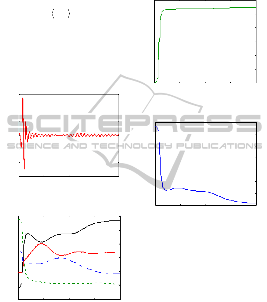
Figures 1 to 4, in which Figure 1 shows the control
field. The corresponding evolution populations of
energy levels 1 through 4 are shown in Figure 2,
from which one can see that the populations are
inverted, i.e., the most energetic state
4 has the
highest population, and the second one has the
second highest population, etc. The final populations
of energy levels are 0.1547, 0.1927, 0.2680, and
0.3845, respectively. Figure 3 shows the
performance index, and Figure 4 shows the distance
from the target state. At the target time, the distance
is
2
ˆˆ
0.0034
f
ρρ −= , so that the mixed-state
control is completed. In Ref. Schirmer, et al. (2000)
OPTIMAL CONTROL OF MIXED-STATE QUANTUM SYSTEMS BASED ON LYAPUNOV METHOD
27

0
ˆ
ˆ
AH= , and at the target time 200 a.u.
f
t = the
expectation value
ˆ
()
f
A
t is 99% of the
theoretical maximum. While in this paper, this ratio
is also 99% . Under the condition that the
simulation result is the same, the design process of
the control law in this paper is easier than that in
Ref. Schirmer, et al. (
2000) which needs iteration.
Also, by comparing the results, we can find that the
inverted rate of the levels is faster here, that is
because the initial control value is larger. In the real
applications, the control value can be tuned
according to the requirement.

0 50 100 150 200
-0.45
-0.3
-0.15
0
0.15
0.3
0.45
Time (a.u.)
Field (a.u.)
Figure 1: Optimal control field for a four-level Morse
oscillator model.

0 50 100 150 200
0.1
0.15
0.2
0.25
0.3
0.35
0.4
Time (a.u.)
Populations
|4>
|3>
|2>
|1>
Figure 2: Evolution of populations for a four-level Morse
oscillator model.

0 50 100 150 200
0
0.1
0.2
0.3
0.4
0.5
0.6
Time (a.u.)
Index
Figure 3: Performance index for a four-level Morse
oscillator model.

0 50 100 150 200
0
0.02
0.04
0.06
0.08
0.1
0.12
0.14
Time (a.u.)
Distance
Figure 4: Distance from target state for a four-level Morse
oscillator model.
4.2 Harmonic Oscillator Model
Comparing with the above mentioned completely
controllable Morse oscillator model, here we
consider the diatomic molecule described by a four-
level Harmonic oscillator model. The vibrational
energy levels are determined by
1
2
n
En
=
−
(28)
Thus the energy levels are
1
0.5E = ,
2
1.5E = ,
3
2.5E = and
4
3.5E = . The dipole moments in
this model are 1
n
d
=
, ( 1, 2,3)n = . The system is
not completely controllable because the dimension
of the Lie algebra generated by
0
ˆ
H
and
1
ˆ
H
is less
than 16 (
Barnett and Dalton, 1987). We still suppose
BIOSIGNALS 2011 - International Conference on Bio-inspired Systems and Signal Processing
28

that the initial density is
4
0
1
ˆ
n
n
wnn ρ
=
=
∑
, in
which
1
0.3850w = ,
2
0.2758w = ,
3
0.1976w =
and
4
0.1416w = . The target state and the control
law are the same as that in the situation of the Morse
oscillator model. Starting with
0
0.15a.u.f = ,
0.1a.u.dt = ,
1
1r = , and
(4,1,1,1,1,3,1,1,1,1,2,1,1,1,1,1)Pdiag= , the
simulation curves are shown in Figures 5-8. At the
target time, the populations of energy levels are
0.1482, 0.2003, 0.2732, and 0.3783, respectively,
and the distance from the target state is
2
ˆˆ
0.0036
f
ρρ −= . Despite the system is not
completely controllable, the method in this paper is
still efficient.

0 50 100 150 200
-0.12
-0.08
-0.04
0
0.04
0.08
0.12
Time (a.u.)
Field (a.u.)
Figure 5: Optimal control field for a four-level Harmonic
oscillator model.

0 50 100 150 200
0.1
0.15
0.2
0.25
0.3
0.35
0.4
Time (a.u.)
Populations
|4>
|3>
|2>
|1>
Figure 6: Evolution of populations for a four-level
Harmonic oscillator model.
0 50 100 150 200
0
0.03
0.06
0.09
0.12
0.15
0.18
Time (a.u.)
Index
Figure 7: Distance from target state for a four-level
Harmonic oscillator model.
5 CONCLUSIONS
In this paper we have developed an optimal control
method based on Lyapunov theorem for the
Liouville equation to realize the quantum control of
the mixed states. The detailed design processes of
the control laws have been given both in the cases of
the target density operator of the system of interest
being a diagonal form and a general one,
respectively. Moreover, the numerical simulations
were performed for the diatomic molecule described
by the Morse oscillator model. The simulation
results show that the method proposed is as efficient,
even in the case that the system is not completely
controllable.
ACKNOWLEDGEMENTS
This work was supported in part by the National Key
Basic Research Program under Grants No.
2006CB922004 and No. 2009CB929601, the
National Science Foundation of China under Grant
No. 61074050.
REFERENCES
Athans, M. and Falb, P. L., 1966, Optimal Control
McGraw-Hill, New York.
Barnett, S. M. and Dalton, B. J., 1987, Liouville space
description of thermofields and their generalizations,
J. Phys. A: Math. Gen. 20, 411-418.
OPTIMAL CONTROL OF MIXED-STATE QUANTUM SYSTEMS BASED ON LYAPUNOV METHOD
29

Beauchard, K., Coron, J. M., Mirrahimi M. and Rouchon,
P., 2007, Implicit Lyapunov control of finite
dimensional Schrodinger equations,
Systems & Control
Letters
56, 388.
Belavkin, V. P., 1992, Quantum stochastic calculus and
quantum nonlinear filtering,
Journal of Multivariate
Analysis
42, 171-201.
Bouten, L., Mâdâlin Guţâ, and Maassen, H., 2004,
Stochastic Schrodinger equations,
J. Phys. A, 37, 3189.
Cong, S. and Kuang, S., 2007, Quantum control strategy
based on state distance,
Acta Automatica Sinica 33, 28-
31.
D’Alessandro, D. and Dahleh, M., 2001, Optimal control
of two-level quantum systems,
IEEE Transactions on
Automation Control
, 46, 866.
Doherty A. C.andJacobs, K., 1999, Feedback control of
quantum systems using continuous state estimation,
Phys. Rev. A, 60, 2700.
Girardeau, M. D. Schirmer, S. G. Leahy, J. V.and Koch,
R. M., 1998, Kinematical bounds on optimization of
observables for quantum systems,
Phys. Rev. A, 58,
2684.
Grivopoulos, S. and Bamieh, B., 2003, Lyapunov-based
control of quantum systems, in
Proceedings of the
42nd IEEE Conference on Decision and Control
,
Maui, Hawaii USA.
Judson, R. S. and Rabitz, H., 1992, Teaching Lasers to
Control Molecules,
Phys. Rev. Lett. 68, 1500-1503.
Kuang, S. and Cong, S., 2008, Lyapunov control methods
of closed quantum systems,
Automatica 44, 98-108.
Mirrahimi, M. Rouchon, P. and Turinici, G., 2005,
Lyapunov control of bilinear Schršdinger equations,
Automatica 41: 1987.
Nielsen, M. A. and Chuang, I. L., 2000,
Quantum
Computation and Quantum Information
(Cambridge
University Press, England.
Ohtsuki, Y. and Fujimura, Y., 1989,
J. Chem. Phys. 91,
3903.
Ohtsuki, Y. Kono, H. and Fujimura, Y., 1998,
J. Chem.
Phys.
, 109, 9318.
Peirce, A. P. Dahleh, M. A. and Rabitz, H., 1988, Optimal
control of quantum-mechanical systems: Existence,
numerical approximation, and applications,
Phys. Rev.
A,
37, 4950 .
Phan, M. Q.and Rabitz, H., 1999, A self-guided algorithm
for learning control of quantum-mechanical systems,
J.
Chem. Phys.
, 110, 34 -41.
Schirmer, S. G., 2000, Ph.D. thesis, Oregon University.
Schirmer, S. G. Fu, H. and Solomon, A. I., 2001,
Complete controllability of quantum systems,
Phys.
Rev. A
, 63, 063410.
Schirmer, S. G., Girardeau, M. D. and Leahy, J. V., 2000,
Efficient algorithm for optimal control of mixed-state
quantum systems,
Phys. Rev. A, 61, 012101.
Sugawara, M., 2003, General formulation of locally
designed coherent control theory for quantum system
J. Chem. Phys., 118, 6784-6800.
Wang, X. T. And Schirmer, S. G., 2008, Analysis of
Lyapunov Method for Control of Quantum States,
quant-h/0801.0702.
Zhang, C. W. Li, C. F. and Guo, G. C., 2000, Quantum
clone and states estimation for n-state system,
Phys.
Lett. A
, 271, 31-34.
Zhang, Y. Y. and Cong, S., 2008, Optimal quantum
control based on the Lyapunov stability theorem,
Journal of University of Science and Technology of
China
38, 331-336.
BIOSIGNALS 2011 - International Conference on Bio-inspired Systems and Signal Processing
30