DISULFIDE CONNECTIVITY PREDICTION WITH EXTREME

LEARNING MACHINES

Monther Alhamdoosh, Castrense Savojardo, Piero Fariselli and Rita Casadio

Biocomputing Group, University of Bologna, Via Irnerio 42, 40127 Bologna, Italy

Keywords:

Disulﬁde connectivity, Disulﬁde bonds, Extreme learning machine, Backpropagation, ELM outperforms BP,

Multiple feature vectors, Disulﬁde proteins, Disulﬁde bridge prediction, K-mean clustering with ELM, RBF

networks with ELM, SLFN with ELM.

Abstract:

Our paper emphasizes the relevance of Extreme Learning Machine (ELM) in Bioinformatics applications by

addressing the problem of predicting the disulﬁde connectivity from protein sequences. We test different

activation functions of the hidden neurons and we show that for the task at hand the Radial Basis Functions

are the best performing. We also show that the ELM approach performs better than the Back Propagation

learning algorithm both in terms of generalization accuracy and running time. Moreover, we ﬁnd that for the

problem of the prediction of the disulﬁde connectivity it is possible to increase the predicting performance by

initializing the Radial Basis Function kernels with a k-mean clustering algorithm.

Finally, the ELM procedure is not only very fast but the ﬁnal predicting networks can achieve an accuracy of

0.51 and 0.45, per-bonds and per-pattern, respectively. Our ELM results are in line with the state of the art

predictors addressing the same problem.

1 INTRODUCTION

The prediction of protein structures from their se-

quences is still an open problem in Structural Bioin-

formatics, especially considering that the dispropor-

tion between the huge number of putative protein se-

quences with respect to the smaller number of known

3D structures. Over the last two decades several ap-

proaches were described in order to ﬁnd approximate

solutions to the protein folding problem and tools

have been developed to facilitate the search of a likely

structural template for the protein sequence at hand.

Among these, the identiﬁcation of the correct pairing

of bonded cysteines in the protein sequence (disulﬁde

connectivity) helps in constraining its folded struc-

ture.

The problem of the prediction of disulﬁde connec-

tivity can be logically split into two steps: 1) predict-

ing the disulﬁde-bonding state (namely the identiﬁca-

tion of the cysteine residues that in the protein chain

are/are not likely to make disulﬁde bonds); 2) assign-

ing the connectivity pattern of the bonded cysteines.

For the ﬁrst step several methods are available and

achieve an average per-protein accuracy higher than

80% (Muskal et al., 1990; Fiser et al., 1992; Fariselli

et al., 1999; Fiser and Simon, 2000; Mucchielli-

Giorgi et al., 2002; Martelli et al., 2002; Chen et al.,

2004; Liu, 2007). Finding solutions for the second

step is generally harder than for the ﬁrst one, since

cysteine pairing in the protein space is a problem

of global optimization in the protein feature space

and the bridge formation is not necessarily depen-

dent on local functional and structural motifs. Ma-

chine learning and computational methods have been

widely used to solve the disulﬁde connectivity pre-

diction problem over the past years with signiﬁcant

progresses.

Fariselli and Casadio (2001) ﬁrst addressed the

prediction of disulﬁde connectivity as a combinatorial

optimization problem that ﬁnds the maximum-weight

perfect matching of a complete undirected weighted

graph. According to this graph model vertices are

the putative bonded cysteines and edges represent

the strength of interactions among corresponding cys-

teine pairs. Since the graph is complete, the Edmond-

Gabows (EG) algorithm (Gabow, 1975) is the most

suitable method to solve the corresponding Linear

Programming problem. The weight edges were com-

puted using stochastic optimization methods (Fariselli

and Casadio, 2001) or neural networks (Fariselli et al.,

2002; Shi et al., 2008).

Later other methods were developed and these in-

Alhamdoosh M., Savojardo C., Fariselli P. and Casadio R..

DISULFIDE CONNECTIVITY PREDICTION WITH EXTREME LEARNING MACHINES.

DOI: 10.5220/0003125600050014

In Proceedings of the International Conference on Bioinformatics Models, Methods and Algorithms (BIOINFORMATICS-2011), pages 5-14

ISBN: 978-989-8425-36-2

 2011 SCITEPRESS (Science and Technology Publications, Lda.)

clude a bi-recursiveneural network system (Vullo and

Frasconi, 2004), a method based on Cysteine Separa-

tion Proﬁles (CSPs) (Zhao et al., 2005), neural net-

works that exploit diresidue composition (Ferr`e and

Clote, 2005), two dimensional recursive neural net-

works (Baldi et al., 2005), K-nearest neighbors algo-

rithm (Chen et al., 2006), support vector regression

(Song et al., 2007; Zhu et al., 2010), support vec-

tor machines (Lu et al., 2007), statistical analysis in-

cluding correlated mutations (Rubinstein and Fiser,

2008), decomposition convolution kernels (Vincent

et al., 2008) and recently prediction based on com-

parative modeling (Lin and Tseng, 2010).

Although it is difﬁcult to compare the perfor-

mance of different predictors, often trained and tested

on different protein sets with different levels of ho-

mology, and implementing different protein features,

the present best performance is in the range of 50-

60% per protein accuracy depending on the num-

ber of disulﬁde bridges. In any case all the above

approaches are poorly performing when the num-

ber of bridges in the protein is ≥5. This was/and

still remains due to the paucity of examples in the

PDB database of proteins with a large number (≥5)

of disulﬁde bridges included in the training/testing

set. In most of the neural network based methods

quoted above the networks were modeled as directed

acyclic graphs (DAG) trained with the very popu-

lar back-propagation (BP) algorithm that implements

the steepest gradient descent (GD) search through the

space of network weights. Trapping in local minima

is one of the major problem of this procedure and

the search in the weights space is generally slow and

time-consuming, especially considering that the num-

ber of training examples in the biological data bases

is exponentially increasing and methods need learn-

ing updating.

In this paper, we are approaching the problem of

disulﬁde connectivity prediction using single-hidden

layer feed-forwardneural network (SLFN), with a lat-

est machine learning technology called the Extreme

Learning Machine (ELM) (Huang et al., 2004). We

investigate the performanceof this algorithm with dif-

ferent activation functions as compared to the classi-

cal BP approach. We ﬁnd that the ELM procedure

is very fast and that the ﬁnal predicting networks can

achieve an accuracy of 0.51 and 0.45, per-bonds and

per-pattern respectively. Our ELM results are there-

fore in line with the state of the art predictors address-

ing the same problem and are obtained with less com-

putational time.

The remainder of the paper is organized as fol-

lows: Section 2 describes the ELM learning algo-

rithm. Section 3 presents our dataset and the exper-

imental protocol of our work. Section 4 shows and

discusses results, and concludes this paper.

2 BRIEF OF THE EXTREME

LEARNING MACHINE

Single-hidden layer feed-forward neural network

(SLFN) have been showed to be sufﬁcient to solve

very difﬁcult mapping (Huang, 2003; Tamura and

Tateishi, 1997). However, traditional learning al-

gorithms for feed-forward networks, like back-

propagation, require tuning many parameters over an

iterative procedure that is very time-consuming. To

overcome this issue, in the recent years the Extreme

Learning Machines have been introduced (Huang

et al., 2006b; Huang et al., 2004; Huang and Siew,

2004; Huang and Siew, 2005; Huang et al., 2006a).

For sake of clarity we brieﬂy introduce the mathemat-

ical notation used to deﬁne ELM.

2.1 Mathematical Perspective on SLFNs

For N arbitrary distinct samples (x

), where x

,··· ,x

]

∈ R

and t

= [t

,··· ,t

]

∈ R

, a standard SLFN with N hidden neurons and an ac-

tivation function g(x) is mathematically modeled as

∑

i=1

g(w

+ b

) = o

, j = 1, · · · ,N (1)

where w

= [w

,··· ,w

]

is the weight vector

connecting the ith hidden neuron and the input neu-

rons, β

= [β

,β

,··· ,β

]

is the weight vector con-

necting the ith hidden neuron and the output neurons,

and b

is the threshold of the ith hidden neuron. w

·x

denotes the inner product of w

and x

. The standard

SLFNs can approximate these N samples with zero

error if there exist β

, w

and b

such that

∑

i=1

g(w

+ b

) = t

, j = 1,··· ,N (2)

The above N equations can be written compactly as:

Hβ = T (3)

where

H(w

,··· ,w

,··· ,b

,··· ,x

) =







g(w

+ b

) ··· g(w

+ b

)

. ···

g(w

+ b

) ··· g(w

+ b

)







N×

(4)

BIOINFORMATICS 2011 - International Conference on Bioinformatics Models, Methods and Algorithms

β =













N×m

and T =













N×m

(5)

H is called the hidden layer output matrix of the neu-

ral network (Huang, 2003); the ith column of H is

the ith hidden neuron output with respect to inputs

,...,x

The same formulation can be extended to Radial

Basis Function (RBF) networks, where each g(w

) in the hidden layer matrix H is substituted with a

RBF kernel:

(x) = φ



kx− µ



(6)

where µ

= [µ

,µ

,...,µ

]

is the ith kernel´s center

and σ

is its impact width.

2.2 ELM Learning Algorithm

Since the number of distinct training examples is usu-

ally much greater than the number of hidden neu-

rons (N ≫

N), the H matrix is a rectangular matrix

and tuning the parameters w

,β

or µ

,σ

,β

(i =

1,...,

N) in order to obtain a unique solution for Hβ =

T is not always possible. Gradient–based learning al-

gorithms try to ﬁnd a solution that minimizes the cost

function

E =

∑

j=1

∑

i=1

) −t

(7)

where f

) is the output of the ith hidden neuron

(additive or RBF kernel) when the training sample x

is introduced to the network.

Seeking simplicity, Huang et al. (Huang et al.,

2004; Huang and Siew, 2004; Huang and Siew, 2005;

Huang et al., 2006a) showed that there is no need to

tune the input weights and biases of hidden neurons

or of the kernel parameters and that they can be ran-

domly set and then ﬁxed. Assuming the input weights

and biases or kernel parameters are ﬁxed, the training

of SLFN is simply ﬁnding a solution

β for the linear

system Hβ = T. Usually this is achieved by adopting

the Moor-Penrose generalized inverse (see theorem in

P.147 of (Serre, 2002)), as:

β = H

†

T (8)

where H

†

is the pseudoinverse matrix of the hidden

layer output matrix H. As analyzed by Huang et

al., this method can reach good generalization per-

formance by ensuring two properties of learning: the

smallest norm of weights besides the smallest squared

error on the training samples, while the gradient-

based algorithms focuses on the later property only.

The three main steps involved in ELM algorithm can

be summarized as:

ELM Algorithm (Huang et al., 2004; Huang and

Siew, 2004). Given a training set D = {(x

)|x

∈

∈ R

,i = 1, . . . ,N}, activation function g or ker-

nel function φ, and number of hidden neurons or ker-

nels

Step 1 Assign randomly input weights w

and biases

for additiveneurons or centers µ

and impact widths

,i = 1, . . . ,

N for RBF kernels.

Step 2 Calculate the hidden layer output matrix H.

Step 3 Calculate the output weights β:

β = H

†

The efﬁciency of this algorithm comes from its

ability to use many nonlinear activation and kernel

functions without restriction for being differential,

and to avoid the troubling issues such as stopping cri-

teria, learning rate, learning epochs and local minima.

3 IMPLEMENTATION AND

METHODS

3.1 Dataset PDB0909

From the Protein Data Bank (PDB) (Berman et al.,

2000), release of September 2009 we retrieved all

protein structures that are resolved by X-ray experi-

ments with resolution between 0 and 2.5 A

◦

. Simi-

lar sequences were removed at 70% identity, then the

chain with longest length and highest resolution for

each protein was selected. To eliminate the redun-

dancy we followed this procedure: an all-against-all

BLAST (Altschul et al., 1990) sequence search was

performed on the starting protein set, then we clus-

tered similar chains together (as connected compo-

nents of an undirected graph) and only the longest

chain of each cluster was retained as representative.

Two protein chains are deﬁned similar if they share a

sequence identity > 25% and an alignment coverage

> 80%. After this basic ﬁltering process, we sorted

out only the protein chains that have at least two intra-

chain bonded cysteines, so that we ended up with 796

chains. In our study, we only focus on the chains that

have 2, 3, 4, and 5 intra-chain disulﬁde bonds since

chains with more than 5 bridges are very few and can-

not be statistically tested (chains with one disulﬁde

bridge are trivial cases). Table 1 shows the number

of chains with 2, 3, 4 and 5 bridges and other statis-

tics about each connectivity size. The % Coverage of

Patterns Space column shows the lack of patterns rep-

DISULFIDE CONNECTIVITY PREDICTION WITH EXTREME LEARNING MACHINES

resentation when the number of bonded cysteines gets

higher than eight.

3.2 Cross-validation Sets

A 4-fold cross-validation procedure was used to eval-

uate the performance of our predictor, in which the

dataset is partitioned into four almost-equal-size sub-

sets. The results obtained for the four tests are com-

bined to produce a single evaluation. In order to

guarantee the absence of homology among the folds

we further re-aligned with BLAST all the sequences

against themselves. We then deﬁned two sequences as

similar if their identity is > 25%. According to this

labeling, similar sequences were then clustered and

chains of the same cluster were assigned to the same

cross-validation fold.

3.3 Measures of Performance

Given a protein primary sequence with N(= 2B) cys-

teines forming B disulﬁde bridges, the number of pos-

sible cysteine pairs is:





2B!

2!(2B− 2)!

= B(2B− 1), (9)

and the number of possible connectivity patterns is:

= (2B− 1)!! =

(2n)!

.n!

(10)

The number of possible connectivity patterns dra-

matically grows as the number of disulﬁde bridges in-

creases. For this reason among the several indexes

that can be used to score the predictions (Ferr`e and

Clote, 2005; Baldi et al., 2005), the most informative

are: the disulﬁde bond index Q

and disulﬁde pattern

index Q

(Fariselli and Casadio, 2001). Q

, globally

evaluates the ability of a predictivesystem to correctly

predict disulﬁde connectivity patterns and is given by:

∑

i=1

(x,y)

, (11)

where δ

(x,y) is equal to 1 if the predicted pattern y of

the ith protein coincides with its correct pattern x and

is the total number of predicted protein chains. In

4-fold cross-validation, we collect the numbers of cor-

rectly predicted patterns from all folds, and then av-

erage them over the size of the un-partitioned dataset.

Alternatively, Q

is a pair-wise index that estimates

the predictive accuracy of individual disulﬁde bonds

i.e. the percentage of disulﬁde bridges that are cor-

rectly predicted, and is given by:

∑

i=1

∑

j=1

(x,y)

, (12)

where δ

(x,y) is equal to 1 if the jth predicted disul-

ﬁde bond y of the ith predicted pattern coincides with

a correct disulﬁde bond x in the correct pattern, B

is the connectivity size of the ith pattern, and T

the total number of possible pairs in the T

proteins.

Similarly, the numbers of correctly predicted pairs are

collected from all folds during cross-validation and

the total Q

value is computed by averaging these

numbers over the total number of pairs in the un-

partitioned dataset.

To score the performance we deﬁne a random pre-

dictor R

without bias a predictor that assigns ran-

domly the bonding pairs. For R

the performances

can be theoretically computed as:

) =

(2B− 1)!!

(13)

) =

B(2B− 1)

2B− 1

(14)

) is vanishing much faster than Q

)

although both depend on the number of disulﬁde

bridges.

3.4 Multiple Feature Vectors

To assign pairwise probabilities we deﬁned vectors

that represent each cysteine pairs and some global

protein descriptors (Song et al., 2007).

Local Descriptors

Evolutionary information: this descriptor consti-

tutes the largest portion of our multiple sequence fea-

ture vectors that it is composed of w∗ 20 ∗ 2 compo-

nents when the neighbor amino acidic residues around

the two cysteine forming disuﬁde bond are comprised

in a window of size w. We evaluate different window

sizes of the cysteine local context and found out that

w= 13 (six residues ﬂanking the cysteine at each side)

is the most appropriate value. Each position in the

neighbor environment of cysteines, including the cys-

teine position, is encoded with 20 values that are the

frequencies of each residue at this particular position.

This evolutionary information is obtained using the

PSI-BLAST program (Altschul et al., 1997) from the

multiple sequence alignment portrayed in the form of

position-speciﬁc scoring matrices (PSSM). The PSI-

BLAST was run against the non-redundant database

for 3 iterations with an E-value cutoff of 0.001.

Secondary Structure Information: it is also a key

player in improving the prediction accuracy increas-

ing the training vectors with new informative at-

tributes relative to the local environment of cysteines.

In this paper, the DSSP program (Kabsch and Sander,

BIOINFORMATICS 2011 - International Conference on Bioinformatics Models, Methods and Algorithms

Table 1: The PDB0909 Dataset. % Coverage of Patterns Space represents the percentage of disulﬁde patterns, out of all

possible patterns, that are observed in our dataset. e.g. for B=2, the patterns space contains 3 patterns (C1C2, C3C4), (C1C3,

C2C4), (C1C4, C2C3). % Coverage of Pairs Space represents the same value, but in terms of ordered cysteine pairs. e.g. for

B=2, the pairs space is composed of 6 pairs (C1C2, C1C3, C1C4, C2C3, C2C4, C3C4).

Connectivity

Size (B)

# of

Chains

# of Bonded

Cysteines

# of Free

Cysteines

Total # of

Cysteines

% Coverage of

Patterns Space

% Coverage of

Pairs Space

2 146 584 103 687 100 100

3 104 624 60 684 100 100

4 52 416 20 436 25.71 100

5 40 400 17 417 3.39 84.44

Total 342 2024 200 2224 7.21 92.55

1983) was used to obtain the secondary structure in-

formation which was encoded into a 3-letters repre-

sentation. The letter A represents the alpha helix (H),

3-helix (G) and 5 helix (I) from the DSSP output, the

letter B encodes for the residues in isolated bridges

(B) and extended strands (E) in the DSSP output, and

ﬁnally the letter C stands for the hydrogen bonded

turns (T), the bends (S) and the loops and irregular el-

ements (blank). Technically, each letter was encoded

by three binary bits: 100 for A, 010 for B, 001 for

C and 000 for X (empty place). This descriptor con-

tributes 39 components (13∗3) for each training vec-

tor when w = 13.

Global Descriptors

Residues Composition: it describes the residues

content in a protein sequence as 20-dimensions vec-

tor of the relative frequencies of residues of different

types. These dimensions can be mathematically for-

mulated as following:

;i = 1, . . . , 20 (15)

where n

is the number of occurrences of the residues

of type i in the sequence and L is the length of the

protein sequence.

Protein Sequence Length: when considering a

protein i with

residues from a proteins dataset, the

normalized protein length L

is given by:

−

(16)

where the mean protein length

L and the standard de-

viation SD of protein lengths are computed on the

whole dataset.

Protein Molecular Weight: similarly to the equa-

tion above, for a protein i with M

total molecular

weight we normalized the value as:

−

(17)

where the mean molecular weight

M and the standard

deviation SD are computed on the whole dataset. The

Figure 1: The testing accuracy of prediction when using ad-

ditive neurons and training different connectivity sizes to-

gether. The red, blue, green and magenta curves represent

the accuracies for 2, 3, 4 and 5 connectivty sizes, repsec-

tively. The black curve represents the overall accuracy re-

gardless of the connectivity size.

molecular weight values for the single residues are

taken from ProtScale (Gasteiger et al., 2005).

Cysteines Separation Distance: we coded the cys-

teine sequence separation as:

SEP(C

) = log(| j − i|) (18)

where i and j are the sequence positions of cysteines

and C

, respectively.

Relative Order of Cysteines: this feature en-

codes for two different values of the input vec-

tor, representing the normalized relative order of

the two cysteines. For instance, given a pro-

tein P with 4 cysteines (C

) the cor-

responding normalized ordered list of cysteine is

(1/4,2/4,3/4, 4/4) = (0.25,0.5,0.75,1). So that

when the method train/predict a pair of cysteines the

two corresponding values are taken from the list (e.g.

the pair [C

] is encoded as [0.5,0.75]).

As a result, the ﬁnal training/testing vectors consist

of 623 components based on these protein sequence

features.

DISULFIDE CONNECTIVITY PREDICTION WITH EXTREME LEARNING MACHINES

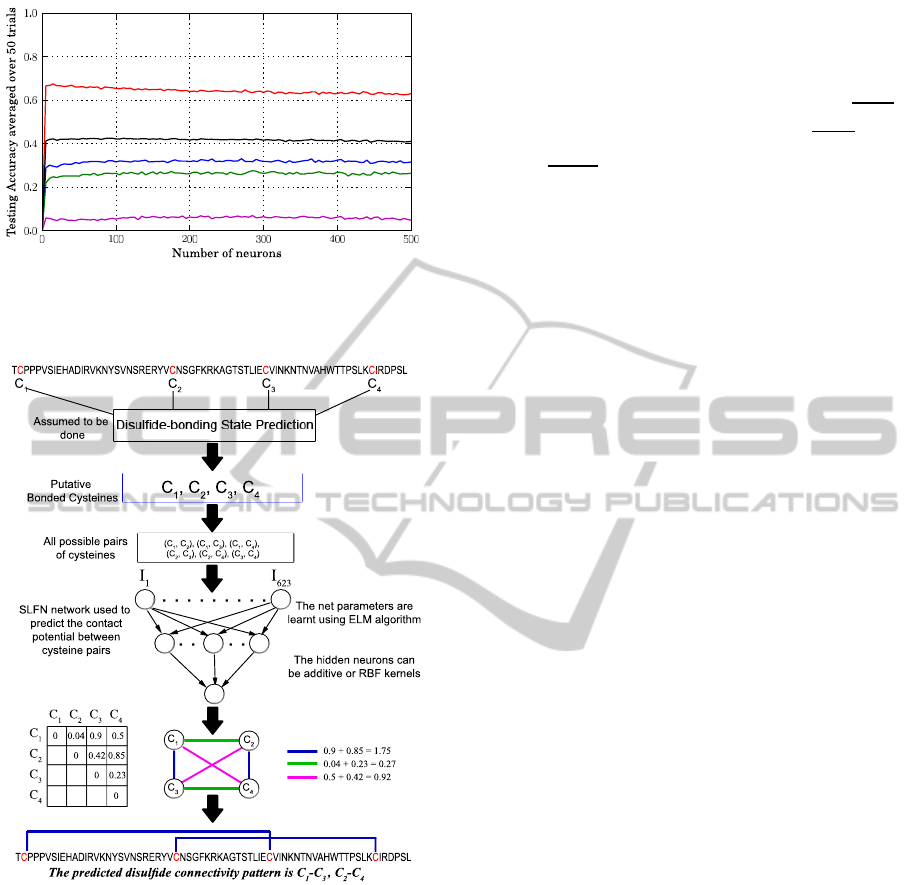
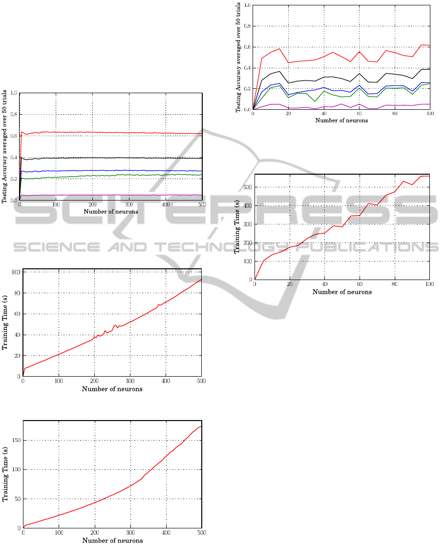
Figure 2: The testing accuracy of prediction when using

L1 RBF kernels and training different connectivity sizes to-

gether.

Figure 3: The general scheme of our proposed disulﬁde

connectivity prediction method. The steps of our procedure

have been illustrated for the chain F of Interleukin-15 re-

ceptor protein whose PDB ID 2PSM.

3.5 Experimental Protocol

The implementation of the proposed model (see Fig-

ure 3) was done using the free scripting language

Python 2.6 (Van Rossum et al., 1991) along with its

numerical package Numpy 1.3 (Oliphant, 2006), used

to compute the pseudo-inverse matrix of the matrix

H in the ELM learning algorithm. Single experi-

ment with different numbers of additive and kernel

hidden neurons have been carried out to ﬁnd the best

estimation of the hidden layers size. Since some of

the network parameters are randomly initialized, each

experiment was run 50 times and then the average

measurementswere taken to evaluate the performance

of our Model. The additive neurons were activated

using the sigmoid activation function g(x) =

1+e

−x

while two Gaussian functions L

(x) = e

−kx−µk

and

(x) = e

−kx−µk

were tested for the RBF kernels. Fur-

thermore, one output neuron was used in most of the

experiments unless otherwise mentioned. We also ex-

amined the performance of the Backpropagation (BP)

learning algorithm on SLFNs with a symmetric sig-

moid activation function for the hidden layer and a

sigmoid activation function for the output layer. The

learning rate was set to 0.1 and MSE threshold error to

0.0001. Interestingly, early stopping condition based

on the accuracy of validation sets has been also em-

ployed to avoid overﬁtting of training data and reduce

training time. The online incremental approach was

used to update weights.

The simulations were executed on a computer of

8 processors, each one with 2.5 GHz frequency, and

16 GB of RAM.

4 RESULTS AND DISCUSSION

We ﬁrst evaluate the SLFN performance as a function

of the number of hidden units adopting a four-fold

cross validation procedure. The results at increasing

number of additive neurons are reported in Figure 1

for the disulﬁde pattern index Qp. Similar graphs re-

porting the Qp values are shown in Figures 2 and 4

when the transfer function during the learning phase

is the Gaussian function with L1 and L2 norms. In

all reported cases, the SLFN performance reaches a

plateau when the number of hidden neuron is larger

than 100. It is worth noticing that the training time

is nearly a linear function of the number of hidden

neuronsirrespectively of the transfer function adopted

(Figure 5). The accuracy index Qp when plotted as a

function of the number of hidden units obtained with

the Back Propagation (BP) learning algorithm is less

stable then that obtained with the EML learning (com-

pare Fig.1,2,4 with Figure 6). Furthermore, the BP

training time as a function of the number of hidden

neurons shows a signiﬁcantly steeper slope with re-

spect to the ELM approach (compare Figures 5(a) and

5(b) with Figure 7). These results highlight the ef-

fective time saving of ELM with respect to BP when

training is performed. The detailed results for the best

performing number of neurons for the different SLFN

models are reported in Table 2, where it is listed that

the RBF networks with L1 function achieve the best

BIOINFORMATICS 2011 - International Conference on Bioinformatics Models, Methods and Algorithms

overall performance both in term of Qc and Qp . This

picture holds also when the performance is evaluated

separately for each subset comprising proteins with a

different number of disulﬁde bonds (Table 2). Table

2 reports also the required learning time, and it ap-

pears that the Back Propagation (BP) algorithm is far

slower than the ELM algorithm.

Figure 4: The testing accuracy of prediction when using

L2 RBF kernels and training different connectivity sizes to-

gether.

(a) Additive hidden neurons.

(b) RBF hidden neurons.

Figure 5: The training time of SLFNs over 4-folds cross-

validation procedure when training different connectivity

sizes together.

Figure 6: The testing accuracy of prediction when using BP

learning algorithm and training different connectivity sizes

together.

Figure 7: The training time of SLFNs over 4-folds cross-

validation procedure when using BP learning algorithm and

training different connectivity sizes together.

4.1 Performance Enhancement

Instead of random initializing the ﬁrst layers of

weights, we select them using a standard K-mean

clustering approach to set the centers and impact

widths of kernels. The value of the selected number of

clusters K corresponds to the number of hidden neu-

rons. Next, for each hidden kernel its center is set by

the center of a cluster while its impact width is set

as the standard deviation of the cluster vectors from

its center. The performance of ELM with L1 Gaus-

sian functions and K-mean clustering algorithm is re-

ported in Figure 8 for Qp. The training time is dom-

inated by the K-mean clustering procedure and can

be several times greater than the random initialization

(compare Figure 9 with Figure 5). This is particu-

lar evident by considering that the K-mean clustering

running time increases with the number of clusters

(K) up to a given threshold that depends on the ratio

between the number of data and the K value.

Then the training time as a function of the num-

ber of hidden neurons decreases (Figure 9), becom-

ing constant when K equates the number of elements

to cluster. Nonetheless, the best results obtained by

DISULFIDE CONNECTIVITY PREDICTION WITH EXTREME LEARNING MACHINES

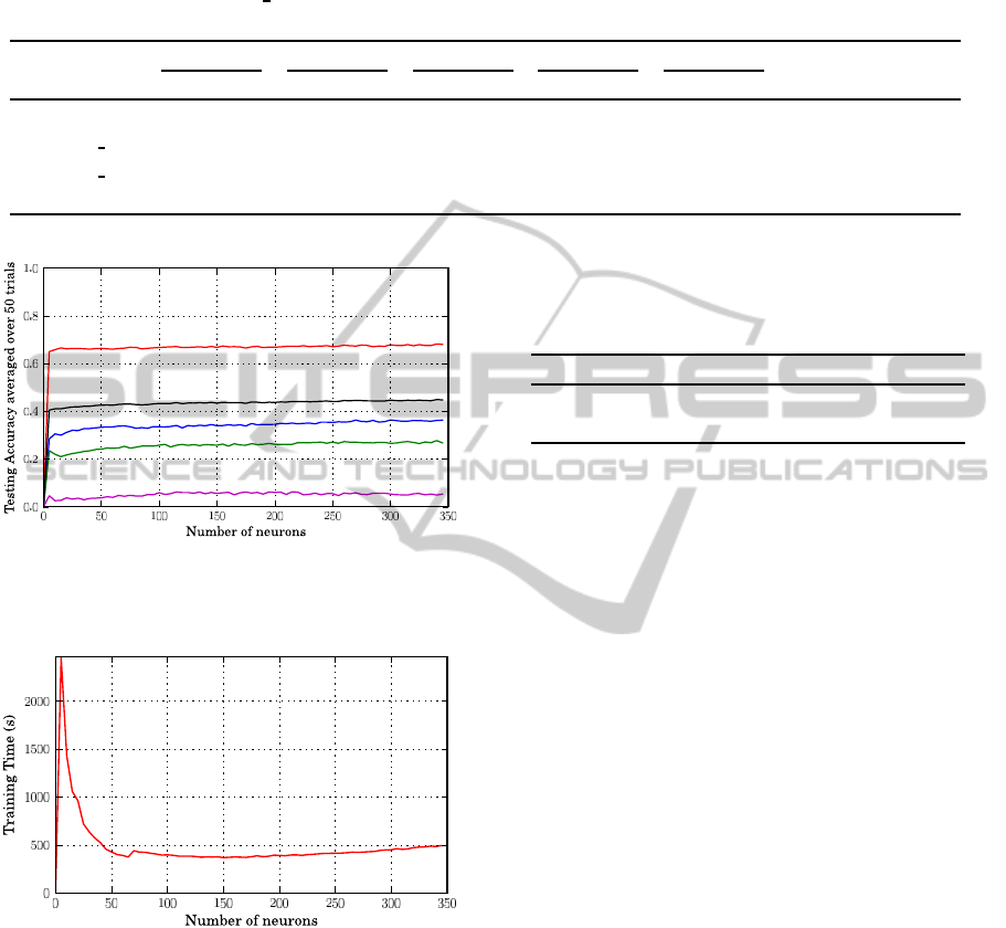
Table 2: Comparison of different ELM-trained models with BP-trained model when different connectivity sizes are trained

together. N

is the best number of hidden neurons (when additive) and kernels (when RBF). Qc and Qp (%) have been

thoroughly explained earlier. ELM (Sig) is a neural network trained with ELM algorithm using sigmoid activation function

for the hidden neurons. ELM (L

RBF) is an RBF neural network trained with ELM algorithm using L

Gaussian function.

Time (s) is the average training time, given in seconds, of 50 experiments.

Model

B = 2 B = 3 B = 4 B = 5 Overall Best # of

neurons

Time

(s)Q

ELM (Sig) 65 65 42 28 42 24 27 4 46 41 150 28.52

ELM (L

RBF) 66 66 45 32 45 26 31 5 48 43 90 18.55

ELM (L

RBF) 64 64 42 28 39 22 28 5 45 40 95 18.55

BP 62 62 38 26 40 23 29 5 44 38 95 559.29

Figure 8: The testing accuracy of prediction when using K-

Mean clustering algorithm to initialize L1 RBF kernels and

training different connectivity sizes togehther.

Figure 9: The training time of SLFNs over 4-folds cross-

validation procedure when using K-mean clustering algo-

rithm to initialize RBF kernels and training different con-

nectivity sizes together.

using the K-mean clustering initialization are slightly

better than the random initialization approach (Table

3).

4.2 Comparison with some Previous

Works

As mentioned in the introduction it is not easy to com-

pare our results with those obtained before, since dif-

Table 3: Our method performance with L1 RBF kernels ini-

tialized using k-mean clustering. The best number of hid-

den neurons is 270 and the corresponding training time is

425.11 seconds.

Connectivity Size 2 3 4 5 overall

67 48 44 37 51

67 36 27 6 45

ferent authors adopted different datasets (sometimes

without reducing the sequence identity between train-

ing and testing sets). Nonetheless for sake of clarity

in Table 4 we compare our best ELM cross-validation

performance with the Random predictor R

, the his-

torical benchmark Fariselli et al. 2002, and two state

of the art methods Vullo and Frasconi (2004) and

Baldi et al. (2005). It is evident that all the meth-

ods perform better than the random predictor and that

the ELM approach compare very well with the state

of the art methods making it a fast and efﬁcient al-

ternative when the problem of the prediction of the

disulﬁde connectivity is addressed.

5 CONCLUSIONS

In this paper we address the problem of the prediction

of the disulﬁde connectivity using an Extreme Learn-

ing Machine approach. We test different activation

functions of the hidden neurons and different way of

initializing the ﬁrst layer of weights. We also evalu-

ate the performance of the different methods both in

term of accuracy and running times. We show that

the ELM learning is faster and generalizes better than

the corresponding Back Propagation training. Among

our tested models we verify that the RBF neural net-

works trained with an ELM procedure are the best

performing approach for the task at hands. We ﬁnd

that a K-mean clustering procedure to select the ﬁrst

layer of weights, improves the overall EML accuracy

BIOINFORMATICS 2011 - International Conference on Bioinformatics Models, Methods and Algorithms

Table 4: Comparison with previous works on disulﬁde connectivity prediction. These results were generated on a benchmark

dataset called SP39 (Fariselli and Casadio, 2001).

Proposed Method

B = 2 B = 3 B = 4 B = 5 Overall

33 33 20 7 14 1 11 0 19 10

Fariselli et al. (2002) 68 68 37 22 37 20 26 2 42 34

Vullo and Frasconi. (2004) 73 73 51 41 37 24 30 13 49 44

Baldi et al. (2005) 74 74 61 51 44 27 41 11 56 49

ELM 72 72 45 33 49 31 44 22 52 45

and that the trained neural system well compares with

the state of the art methods.

ACKNOWLEDGEMENTS

The authors would like to acknowledge Dr. Dianhui

Wang, from the Department of Computer Science and

Computer Engineering at La Trobe University in Aus-

tralia, for his valuable suggestions to utilize ELMs for

the problem at hand.

REFERENCES

Altschul, S. F., Gish, W., Miller, W., Myers, E. W., and

Lipman, D. J. (1990). Basic local alignment search

tool. Journal of Molecular Biology, pages 403–410.

Altschul, S. F., Madden, T. L., Schaffer, A. A., Zhang,

J., Zhang, Z., Miller, W., and Lipman, D. J. (1997).

Gapped blast and psi-blast: a new generation of pro-

tein database search programs. Nucleic Acids Re-

search, 25(17):3389–3402.

Baldi, P., Cheng, J., and Vullo, A. (2005). Large-scale pre-

diction of disulphide bond connectivity. In Saul, L.,

Weiss, Y., and Bottou, L., editors, Advances in Neural

Information Processing Systems, 17, pages 97–104.

MA MIT Press.

Berman, H. M., Westbrook, J., Feng, Z., Gilliland, G., Bhat,

T. N., Weissig, H., Shindyalov, L. N., and Bourne,

P. E. (2000). The protein data bank. Nucleic Acids

Research, 28(1).

Chen, G., Deng, H., Gui, Y., Pan, Y., and Wang, X. (2006).

Cysteine separations proﬁles on protein secondary

structure infer disulﬁde connectivity. In IEEE Inter-

national Conference on Granular Computing.

Chen, Y., Lin, Y.-S., Lin, C.-J., and Hwang, J.-K. (2004).

Prediction of the bonding states of cysteines using

the support vector machines based on multiple fea-

ture vectors and cysteine state sequences. Proteins,

55:1036–1042.

Fariselli, P. and Casadio, R. (2001). Prediction of disulﬁde

connectivity in proteins. Bioinformatics, 17(10):957–

964.

Fariselli, P., Martelli, P. L., and Casadio, R. (2002). A

neural network-based method for predicting the disul-

ﬁde connectivity in proteins. In Damiani, E., edi-

tor, Knowledge Based Intelligent Information Engi-

neering Systems and Allied Technologies (KES), pages

464–468. Amsterdam IOS Press.

Fariselli, P., Riccobelli, P., and Casadio, R. (1999). Role of

evolutionary information in predicting the disulﬁde-

bonding state of cysteine in proteins. Proteins,

36:340–346.

Ferr`e, F. and Clote, P. (2005). Disulﬁde connectivity

prediction using secondary structure information and

diresidue frequencies. Bioinformatics, 21(10):2336–

2346.

Fiser, A., Cserzo, M., Tudos, E., and Simon, I. (1992). Dif-

ferent sequence environments of cysteines and half

cystines in proteins: Application to predict disulﬁde

forming residues. FEBS, 302(2):117–120.

Fiser, A. and Simon, I. (2000). Predicting the oxidation state

of cysteines by multiple sequence alignment. Bioin-

formatics, 16(3):251–256.

Gabow, H. N. (1975). An efﬁcient implementation of ed-

monds al- gorithm for maximum weight matching on

graphs. Technical Report CU-CS-075-75, Department

of Computer Science, Colorado University.

Gasteiger, E., Hoogland, C., Gattiker, A., Duvaud, S.,

Wilkins, M. R., Appel, R. D., and Bairoch, A. (2005).

Protein identiﬁcation and analysis tools on the expasy

server. In Walker, J. M., editor, The Proteomics Pro-

tocols Handbook, pages 571–607. Humana Press.

Huang, G.-B. (2003). Learning capability and storage

capacity of two-hidden-layer feedforward networks.

IEEE Transaction on Neural Networks, 14(2).

Huang, G.-B. and Siew, C.-K. (2004). Extreme learning

machine: Rbf network case. In he Proceedings of the

Eighth International Conference on Control, Automa-

tion, Robotics and Vision (ICARCV).

Huang, G.-B. and Siew, C.-K. (2005). Extreme learning

machine with randomly assigned rbf kernels. Interna-

tional Journal of Information Technology, 11(1):16–

24.

Huang, G.-B., Zhu, Q.-Y., and Siew, C.-K. (2004). Extreme

learning machine: A new learning scheme of feedfor-

ward neural networks. In Proceedings of International

Joint Conference on Neural Networks (IJCNN).

DISULFIDE CONNECTIVITY PREDICTION WITH EXTREME LEARNING MACHINES

Huang, G.-B., Zhu, Q.-Y., and Siew, C.-K. (2006a). Ex-

treme learning machine: Theory and applications.

Neurocomputing, 70:489–501.

Huang, G.-B., Zhu, Q.-Y., and Siew, C.-K. (2006b). Real-

time learning capability of neural networks. IEEE

Transaction on Neural Networks, 17(4):251255.

Kabsch, W. and Sander, C. (1983). Dictionary of protein

secondary structure: pattern recognition of hydrogen-

bonded and geometrical features. Biopolymers,

22(12):2577–2637.

Lin, H.-H. and Tseng, L.-Y. (2010). Dbcp: a web server

for disulﬁde bonding connectivity pattern prediction

without the prior knowledge of the bonding state of

cysteines. Nucleic Acids Research, 38:503–507.

Liu, H.-L. (2007). Recent advances in disulﬁde connectivity

predictions. Bioinformatics, 2:31–47.

Lu, C.-H., Chen, Y.-C., Yu, C.-S., and Hwang, J.-K. (2007).

Predicting disulﬁde connectivity patterns. Proteins,

67:262–270.

Martelli, P. L., Fariselli, P., Malaguti, L., and Casadio,

R. (2002). Prediction of the disulﬁde bonding state

of cysteines in proteins with hidden neural networks.

Protein Engineering, 15(12):951–953.

Mucchielli-Giorgi, M., Hazout, S., and Tuffery, P. (2002).

Predicting the disulﬁde bonding state of cysteines us-

ing protein descriptors. Proteins, 46:243–249.

Muskal, S., Holbrook, S., and Kim, S. (1990). Prediction

of the disulﬁde-bonding state of cysteine in proteins.

Protein Engineering, 3(8):667–672.

Nguyen, D. and Widrow, B. (1990). Improving the learning

speed of 2-layer neural networks by choosing initial

values of the adaptive weights. In Proceedings of the

International Joint Conference on Neural Networks,

volume 3, pages 21–26.

Oliphant, T. E. (2006). Guide to numpy.

Pavelka, A. and Proch´azka, A. (2004). Algorithms for

initialization of neural network weights. In Sborn´ık

pr´ıspevku 12. rocn´ıku konference MATLAB, 2:453–

459.

Rubinstein, R. and Fiser, A. (2008). Predicting disulﬁde

bond connectivity in proteins by correlated mutations

analysis. Bioinformatics, 24(4):489–504.

Serre, D. (2002). Matrices: Theory and applications.

Springer-Verlag New York, Inc.

Shi, O., Cai, C., Yang, H., and Yang, J. (2008). Disulﬁde

bond prediction using neural network and secondary

structure information. The 2nd International Confer-

ence on Bioinformatics and Biomedical Engineering

(ICBBE).

Song, J.-N., Yuan, Z., Tan, H., Huber, T., and Burrage, K.

(2007). Predicting disulﬁde connectivity from protein

sequence using multiple sequence feature vectors and

secondary structure. Bioinformatics, 23(23):3147–

3154.

Tamura, S. and Tateishi, M. (1997). Capabilities of a four-

layered feedforward neural network: Four layers ver-

sus three. IEEE Transaction on Neural Networks,

8(2):251255.

Van Rossum, G. et al. (1991). Python language website

http://www.python.org/.

Vincent, M., Passerini, A., Labb´e, M., and Frasconi, P.

(2008). A simpliﬁed approach to disulﬁde connec-

tivity prediction from protein sequences. BMC Bioin-

formatics, 9(20).

Vullo, A. and Frasconi, P. (2004). Disulﬁde connectivity

prediction using recursive neural networks and evolu-

tionary information. Bioinformatics, 20:653–659.

Zhao, E., Liu, H.-L., Tsai, C.-H., Tsai, H.-K., Chan, C.-

H., and Kao, C.-Y. (2005). Cysteine separations pro-

ﬁles on protein sequences infer disulﬁde connectivity.

Bioinformatics, 21(8):1415–1420.

Zhu, L., Yang, J., Song, J.-N., Chou, K.-C., and Shen, H.-B.

(2010). Improving the accuracy of predicting disulﬁde

connectivity by feature selection. Journal of Comput-

ing Chemistry, 00(00).

BIOINFORMATICS 2011 - International Conference on Bioinformatics Models, Methods and Algorithms