
COMPLEXITY ANALYSIS OF MASS SPECTROMETRY DATA
FOR DISEASE CLASSIFICATION
USING GA-BASED MULTISCALE ENTROPY
Cuong C. To and Tuan D. Pham
Bioinformatics Research Group, School of Engineering and Information Technology
University of New South Wales, Canberra, ACT 2600, Australia
Keywords: Entropy, Time series, Mass spectrometry, Genetic algorithms.
Abstract: Entropy methods including approximate entropy (ApEn), sample entropy (SampEn) and multiscale entropy
(MSE) have recently been applied to measure the complexity of finite length time series for classification of
diseases. In order to effectively use these entropy methods, parameters such as m, r, and scale factor (in
MSE) are to be determined. So far, there have been no general rules to select these parameters as they
depend on particular problems. In this paper, we introduce a genetic algorithm (GA) based method for
optimal selection of these parameters in a sense that the entropic difference between healthy and pathologic
groups are maximized.
1 INTRODUCTION
Proteomics (Eidhammer et al., 2007) can be seen as
a mass-screening approach to molecular biology,
which aims to document the overall distribution of
proteins in cells, identify and characterize individual
proteins of interest, and ultimately to elucidate their
relationships and functional roles. It is at the protein
level that most regulatory processes take place,
where disease processes primarily occur and where
most drug targets are to be found. The readily
available experimental tools for measurement of
protein expression and characterization by mass
spectrometry-based methods have already made a
significant impact on proteomics.
A revolutionary proteomic technology which has
recently been developed is used to create mass
spectrometry cancer dataset (
Conrads and Zhou, 2003).
In its current state, surface-enhanced laser
desorption/ionization time-of-flight mass
spectrometry (SELDI-TOF MS) is the technology
used to acquire the proteomic patterns to be used in
the diagnostic setting. The principle of SELDI-TOF
works as follows: proteins of interest are captured,
by adsorption, partition, electrostatic interaction or
affinity chromatography on a stationary-phase and
immobilized in an array format on a chip surface.
One of the benefits of this process is that raw
biofluids, such as urine, serum and plasma, can be
directly applied to the array surface. After a series of
binding and washing steps, a matrix is applied to the
array surfaces. The species bound to these surfaces
can be ionized by matrix-assisted laser
desorption/ionization (MALDI) and their mass-to-
charge (m/z) ratios measured by TOF MS. The result
is simply a mass spectrum of the species that bound
to and subsequently desorbed from the array surface.
While the inherent simplicity of the technology has
contributed to the enthusiasm generated for this
approach, the implementation of sophisticated
bioinformatic tools has enabled the use of SELDI-
TOF MS as a potentially revolutionary diagnostic
tool (Eidhammer et al., 2007).
With the advancement of the analytical
techniques toward molecular specificity and
sensitivity, the possibility of discovering new
molecular biomarkers of disease has also increased.
This paper introduces a method based on genetic
algorithm which allows an optimal selection of the
control parameters of the entropy approach such that
it can maximize the difference between the entropy
profiles of mass spectrometry time series of healthy
and disease populations.
5
C. To C. and D. Pham T..
COMPLEXITY ANALYSIS OF MASS SPECTROMETRY DATA FOR DISEASE CLASSIFICATION USING GA-BASED MULTISCALE ENTROPY.
DOI: 10.5220/0003119800050014
In Proceedings of the International Conference on Bio-inspired Systems and Signal Processing (BIOSIGNALS-2011), pages 5-14
ISBN: 978-989-8425-35-5
Copyright
c
2011 SCITEPRESS (Science and Technology Publications, Lda.)

2 ENTROPY METHODS
Entropy methods such as approximate entropy
(ApEn) (
Pincus, 1991), sample entropy (SampEn)
(
Richman and Moorman, 2000), and multiscale entropy
(MSE) (
Costa and Goldberger, 2002) have been used to
measure the complexity or regularity of biological
and physiological time series.
Since the introduction of approximate entropy,
Muniyappa et al. (
Muniyappa, 2007) calculated the
approximate entropy of each individual subject’s
growth hormone concentration time series. The
approximate entropy measured the regularity of
hormone release; a higher value of ApEn reflects a
more disordered pattern of hormone secretion. Lake
et al. (
Lake et al., 2002) used sample entropy to
measure time series regularity of cardiac interbeat
(R-R) interval data records from newborn infants.
Rukhin (
Rukhin, 2000) proposed a new method which
was modified from approximate entropy and applied
to the problem of testing for randomness a string of
binary bits. While both ApEn and SampEn yield
scalar value for the entropy measure, MSE uses
SampEn to obtain various entropy values at different
scales. In MSE, there are two processes namely
“coarse-graining” and entropy computation. The
“coarse-graining” yields a new time series data by
averaging original data points within non-
overlapping windows of increasing length. The new
time series data are then used for estimating the
sample entropy value. The procedure is repeated for
different scales to obtain multiple entropy values.
Multiscale entropy has been applied on various
datasets such as interbeat interval time series, and
DNA sequences (
Costa et al., 2005).
Mathematical formulations of approximate
entropy, sample entropy, multiscale entropy, and
genetic algorithms are briefly described as follows.
2.1 Approximate Entropy (ApEn)
Given a time series of N points, U = {u(j): 1 ≤ j ≤
N}. The series of vectors, xm(i), whose length is m
are derived from the time series, U, given by
)}({)( kiui
m
+=x
(1)
where 0 ≤ k ≤ m – 1 and 1 ≤ i ≤ N – m + 1. The
distance between two such vectors given by
})()(max{)]( ),([ kjukiujid
mm
+−+=xx
(2)
We now define )(rC
m
i
, the probability to find a
vector which differs from
x
m
(i) less than the distance,
r, as:
1
)(
)(
,
+−
=
m
N
iN
rC
rm
m
i
(3)
where )(
,
iN
rm
is the number of vectors, x
m
(j) (with 1
≤ j ≤ N – m + 1), such that rjid
mm
≤)]( ),([ xx . The
distance, r, is a fixed parameter which sets the
“tolerance” of the comparison. The average of the
natural logarithms of the functions, )(rC
m
i
is given
by
1
)](ln[
)(
1
1
+−
=Φ
∑
+−
=
m
N
rC
r
mN
i
m
i
m
(4)
Eckmann and Ruelle (
Eckmann and Ruelle, 1985)
suggested approximating the entropy of the
underlying process as
)]()([limlimlim
1
0
rr
mm
Nmr
+
∞→∞→→
Φ−Φ
(5)
Because of these limits, this definition is not suited
to the analysis of the finite time series derived from
experiments. Pincus (Pincus, 1991) saw that the
calculation of )]()([
1
rr
mm +
Φ−Φ for fixed
parameters m, r, and N had intrinsic interest as a
measure of regularity and complexity. For finite data
set, ApEn is given by
)()(),(ApEn
1
rrrm
mm +
Φ−Φ=
(6)
2.2 Sample Entropy (SampEn)
The difference between ApEn and SampEn is that
the latter does not count self-matches when
estimating conditional probabilities. The scheme for
computing SampEn is described as follows. First, we
define the probability that two sequences match for
m points as
)(rB
m
:
ijmNj
m
N
iN
rB
rm
m
i
≠−≤≤
−−
= and 1 ;
1
)(
)(
,
(7)
m
N
rB
rB
mN
i
m
i
m
−
=
∑
−
=
1
)(
)(
(8)
and the probability that two sequences match for (m
+ 1) points as )(rA
m
ijmNj
m
N
iN
rA
rm
m
i
≠−≤≤
−−
=
+
and 1 ;
1
)(
)(
,1
(9)
BIOSIGNALS 2011 - International Conference on Bio-inspired Systems and Signal Processing
6

m
N
rA
rA
mN
i
m
i
m
−
=
∑
−
=
1
)(
)(
(10)
where )(
,1
iN
rm+
is the number of vectors, x
m+1
(j),
such that rjid
mm
≤
++
)]( ),([
11
xx .
Then, the sample entropy is given by
]
)(
)(
[ln )SampEn(
rB
rA
-m, r
m
m
=
(11)
2.3 Multiscale Entropy
Traditional approaches to measuring the complexity
of biological signals fail to account for the multiple
time scales inherent in such time series (
Costa et al.,
2005). Therefore, multiscale entropy has been
introduced to address this drawback. There are two
processes in multiscale entropy. First, multiple
coarse-grained time series are generated by
averaging original data points within non-
overlapping windows. Each element of the coarse-
grained time series,
)( ju
τ
, is given by
∑
+−=
=
τ
τ
τ
τ
j
ji
iuju
1)1(
)(
1
)(
(12)
where
τ
represents the scale factor and 1 ≤ j ≤ N/
τ
.
In the second process, sample entropy is applied
to the coarse-grained time series, )( ju
τ
, derived
from the first process.
2.4 Genetic Algorithms (GAs)
Genetic algorithms (Mitchell, 2001) are computational
systems that mimic evolution and adaptation of
individuals in environment. That means the next
generation is normally better than the previous one.
Genetic algorithms represent each individual of
population as a chromosome (string); and a
chromosome is one of candidate solutions of
problems. So a chromosome should in some way
contain information about solution that it represents.
Encoding of chromosome depends on the problem
heavily. There are some types of encoding as: binary
encoding each of which is a string of bits 0 or 1. In
value encoding, each chromosome is a sequence of
some values; values can be anything connected to the
problem, such as (real) numbers, chars or any
objects. Each chromosome has a fitness value which
describes how well this solution can solve problem.
The scheme of genetic algorithms is: at the first
step a population of random chromosomes is
generated. Fitness value of each chromosome is
computed at the second step. A new generation is
created by using some operations such as
reproduction, crossover, and mutation based on the
fitness value at the third step. Three above steps are
looped until the criteria are satisfied. The criteria can
be a maximum number of generations allowed to be
run or an additional problem-specific success
predicate which have to be satisfied. The result
solution is the best-so-far chromosome (the best
chromosome appears at any generation).
3 GA–BASED
MULTISCALE ENTROPY
The main idea of GA–based multiscale entropy
(GA–based MSE) is to find parameters of multiscale
entropy: length of vector m, criterion of similarity r,
and scale factor
τ to maximize the entropic
difference between healthy and pathologic groups.
The training set of the algorithm consists of two sub-
groups called healthy (H) and pathologic (P) groups
which are defined by
}U,,U,U{P
}U,,U,U{H
21
21
P
N
PP
H
N
HH
P
H
…
…
=
=
(13)
Where
}1:)({U},1:)({U NjjuNjju
P
i
P
i
H
i
H
i
≤≤=≤≤=
are the i–th time series of healthy and pathologic
group. N
H
and N
P
are number of time series in
healthy and pathologic group.
First, we apply (12) to each time series of H and
P group to generate the coarse-grained time series as
P
j
ji
P
k
P
k
H
j
ji
H
k
H
k
Nkiuju
Nkiuju
≤≤=
≤≤=
∑
∑
+−=
+−=
1 with ; )(
1
)(
1 with ; )(
1
)(
1)1(
,
1)1(
,
τ
τ
τ
τ
τ
τ
τ
τ
(14)
Then, the mean sample entropy (or approximate
entropy) of the coarse-grained time series of H and P
group are given by
COMPLEXITY ANALYSIS OF MASS SPECTROMETRY DATA FOR DISEASE CLASSIFICATION USING
GA-BASED MULTISCALE ENTROPY
7

P
N
i
i
H
N
i
i
N
rm
N
rm
P
H
∑
∑
=
=
=
=
1
*
1
*
),(SampEn
SampEn(P)
),(SampEn
SampEn(H)
(15)
where ),(SampEn rm
i
is the sample entropy of the i–
th coarse-grained time series in H or P group given
by (11).
P
N
i
i
H
N
i
i
N
rm
N
rm
P
H
∑
∑
=
=
=
=
1
*
1
*
),(ApEn
ApEn(P)
),(ApEn
ApEn(H)
(16)
where ),(ApEn rm
i
is the approximate entropy of the
i–th coarse-grained time series in H or P group given
by (6).
We determine parameters m, r, and scale factor
such that these parameters maximize the difference
between the mean entropy of H and P groups.
Mathematically, we have the following nonlinear
programming if we use SampEn
Find [m, r,
τ
] which maximize
2**
]SampEn(P)SampEn(H)[),,( −=
τ
rmf
(17)
Subject to
⎩
⎨
⎧
∈>
Ν∈
Rrr
m
and 0
,
τ
(18)
or we have the following nonlinear programming if
we use ApEn
Find [m, r,
τ
] which maximize
2**
]ApEn(P)ApEn(H)[),,( −=
τ
rmf
(19)
Subject to
⎩
⎨
⎧
∈>
Ν∈
Rrr
m
and 0
,
τ
(20)
Analytical solutions to a nonlinear programming
problem are difficult to obtain. There have been no
closed-form solutions of global optimality for
general nonlinear programming problems (
Hagan et
al., 1995), (Seeger, 2006). In most algorithms, the
formula for the search direction is generally derived
from the Taylor series such as steepest descent,
Newton’s method, conjugate gradient, etc., which is
a “local” approximate to the function (
Hagan et al.,
1995)(Seeger, 2006). For problems concerning global
optimization, genetic algorithms have been
extensively studied. GAs can be considered as a
“globalization technique” because they can handle a
population of candidate solutions. Another advantage
of GAs is that GAs do not use gradients or Hessians
which may not exist or difficult to obtain (Chong and
Zak, 2001). So we decided to use GAs to solve the
above nonlinear programming. We describe the GAs
components employed in this study as follows.
Chromosome Encoding: each chromosome
represents a tri-tuples of two natural numbers and a
real number, [m, r,
τ
]. So each chromosome is
encoded as a fixed-length string of 3 numbers (value
encoding).
Fitness Function: because initial population is
randomly created as a set of tri-tuples of numbers
which satisfy (18), and mutation operation is not
used, so the criteria of (18) are satisfied during
search process. The objective function (17) or (19) is
used to calculated fitness value of each chromosome.
In other word, the objective function (17) or (19) is
the fitness function.
Control Parameters of GAs: based on the results
of (To and Vohradsky, 2007)(To and Vohradsky,
2007) we selected values for the control parameters
of GAs listed in Table 1.
Table 1: Control parameters of gas.
Parameters Values
Number of generation 500
Population size 1000
Probability of crossover 0.9
Probability of reproduction 0.1
4 EXPERIMENTS
4.1 Ovarian Cancer Data
This dataset (Petricoin, 2002) were produced using
the WCX2 protein chip. The goal of this study was
to explore the impact of robotic sample handling
(washing, incubation, etc.) on the spectral quality.
The authors employed an upgraded PBSII SELDI-
TOF mass spectrometer to generate the spectra.
Different sets of ovarian serum samples were used
compared to previous studies. Figs 1 and 2 show the
typical SELDI mass spectrometry of the control and
ovarian cancers samples which were not randomized
BIOSIGNALS 2011 - International Conference on Bio-inspired Systems and Signal Processing
8

so that the authors could evaluate the effect of
robotic automation on the spectral variance within
each phenotypic group. This database has 253
patterns each of which belongs to ovarian cancer
class or control class. Each pattern is a time series
whose length is 15154.
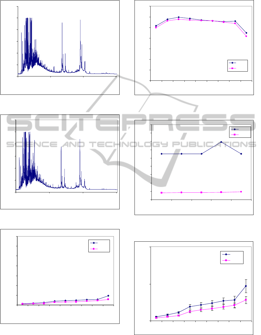
Figs. 3 and 4 show MSE analysis of control
sample and cancer sample whose parameters were
randomly selected using SampEn and ApEn,
respectively. The values plotted in Figs. 3 and 4 are
mean and the standard deviations of these values are
listed in Table 2. If we have a glimpse of Figs. 3 and
4, we see that the separation of two curves is not
good. Therefore, selection of parameters such as m,
r, and scale factor that maximize the separation of
two curves is not trivial task because the cardinality
of the set {m, r, scale factor} is uncountable.
Solving the nonlinear programming (17) or (19)
will give the parameters such as m, r, and scale
factor that maximize the separation of two curves.
Fig. 5 shows the application of GA–based MSE to
ovarian cancer dataset with mean values. The
standard deviations of these mean values are listed in
Table 4 and the parameters of GA–based MSE listed
in Table 3.
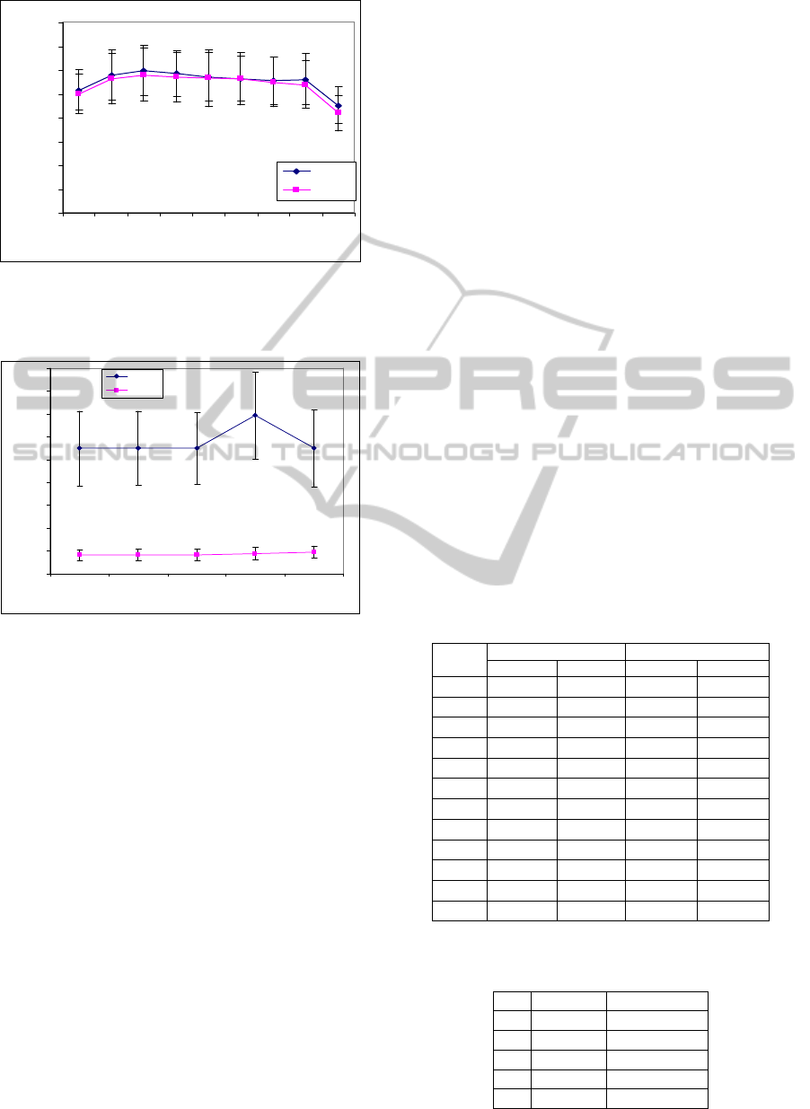
In order to compare the separation of two entropy
curves plotted in Figs. 3, 4, and 5, we can use two
measures: first, we plot mean values ± standard
deviation. Second, we calculate the distance of two
curves using the Euclidean distance formula.
For the first measure, we combine Figs. 3–4 and
Table 2 to plot mean values ± standard deviation of
MSE results as shown in Figs. 6 and 7. The curves of
MSE–ApEn completely overlap while the MSE–
SampEn curves have half of points which do not
overlap but the separations of these points are not as
good as the results of GA–based MSE. We see that
the separations of MSE–SampEn curves are better
that MSE–ApEn curves because SampEn does not
count self-matches so it does not increase conditional
probabilities.
Using Fig. 5 and Table 4, we can plot mean
values ± standard deviation of GA–based MSE
results as shown in Fig. 8 with a very high separation
and no overlapped points. Therefore, the separations
of curves given by GA–based MSE are better than
MSE.
For the second measure which uses the Euclidean
distance to estimate the separation of two entropy
profiles. The distance given by GA–based MSE is
2.22 while 0.10 and 0.10 are the distances given by
MSE–SampEn and MSE–ApEn, respectively. It can
be seen that the distance of GA–based MSE is 22
times further than the distance of MSE.
Large computational time is a drawback of GA–
based methods but it is not in GA–based MSE
because of two reasons. First, if we randomly select
parameters of MSE to maximize the separation of
two entropy curves it takes more time than GA–
based MSE. Second, the above nonlinear
programming (17–18 or 19–20) has no closed–form
solutions so we can not use direct math methods to
solve. Almost search algorithms which are generally
derived from the Taylor series such as steepest
descent, Newton’s method, conjugate gradient, etc.,
is a “local” approximate to the function(Hagan et al.
1995)(Seeger, 2006) and these methods need
gradients or Hessians which is time–intensive to
compute. While GA–based method is a good
candidate because it can be considered as “global”
search and does not need gradients or Hessians of
objective functions.
Although the training process is time-consuming,
the selected parameters are applied many times
without retraining. That means we have one–training
many-usage process.
Table 2: Standard deviation of MSE analysis of ovarian
cancer data.
Scale
factor
SampEn ApEn
Control Cancer Control Cancer
1 0.0037 0.0018 0.1683 0.1679
2 0.0040 0.0026 0.2118 0.2098
3 0.0050 0.0034 0.2114 0.2226
6 0.0112 0.0073 0.1936 0.2054
7 0.0126 0.0083 0.2035 0.2378
8 0.0141 0.0102 0.1896 0.2183
9 0.0162 0.0117 0.1989 0.2068
10 0.0207 0.0145 0.2161 0.2018
30 0.0354 0.0193 0.1535 0.1448
Table 3: Parameters of GA–based MSE of ovarian cancer
data.
M r Scale factor
41 0.47 42
40 0.43 43
39 0.43 44
11 0.07 45
10 0.06 46
Table 4: Standard deviation of GA–based MSE of ovarian
cancer data.
Scale factor Control Cancer
42 0.3270 0.0497
43 0.3245 0.0480
44 0.3147 0.0498
45 0.3797 0.0532
46 0.3381 0.0514
COMPLEXITY ANALYSIS OF MASS SPECTROMETRY DATA FOR DISEASE CLASSIFICATION USING
GA-BASED MULTISCALE ENTROPY
9
0
20
40
60
80
100
120
1 5001 10001 15001
Time index
Relative intensity
Figure 1: Control sample.
0
20
40
60
80
100
120
1 5001 10001 15001
Time index
Relative intensity
Figure 2: Ovarian cancer sample.
0
0.2
0.4
0.6
0.8
1
1.2
1.4
12367891030
Scale factor
SampEn
Control
Cancer
Figure 3: MSE–SampEn analysis of the ovarian cancer
dataset (values are given as means with m = 11, r = 0.073).
0
0.2
0.4
0.6
0.8
1
1.2
1.4
1236 7891030
Scale factor
ApEn
Control
Cancer
Figure 4: MSE–ApEn analysis of the ovarian cancer
dataset (values are given as means with m = 1, r = 0.0567).
0
0.2
0.4
0.6
0.8
1
1.2
1.4
1.6
1.8
42 43 44 45 46
Scale factor
SampEn
Control
Cancer
Figure 5: GA–based MSE analysis of ovarian cancer
dataset (values are given as means).
0
0.2
0.4
12367891030
Scale factor
SampEn
Control
Cancer
Figure 6: MSE–SampEn analysis of the ovarian cancer
dataset (values are given as means ± standard deviation
with m = 11, r = 0.073).
BIOSIGNALS 2011 - International Conference on Bio-inspired Systems and Signal Processing
10
0
0.2
0.4
0.6
0.8
1
1.2
1.4
1.6
12367891030
Scale factor
ApEn
Control
Cancer
Figure 7: MSE–ApEn analysis of the ovarian cancer
dataset (values are given as means ± standard deviation
with m = 1, r = 0.0567).
0
0.2
0.4
0.6
0.8
1
1.2
1.4
1.6
1.8
42 43 44 45 46
Scale factor
SampEn
Control
Cancer
Figure 8: GA–based MSE analysis of ovarian cancer
dataset (values are given as means ± standard deviation).
4.2 MACE Data
This dataset has recently been studied in (Zhou et al.,
2006) (Pham et al., 2008). These authors used high-
throughput, low-resolution SELDI MS to obtain the
protein profiles from patients and controls. Figs 9
and 10 show the typical SELDI mass spectra of the
control and MACE samples, respectively, where the
m/z values are converted to time indexes. The
protein profiles were acquired from 2 to 200 kDa.
Figs. 11 and 12 show SampEn and ApEn curves
of control and MACE samples, respectively using
MSE analysis. Table 5 lists the standard deviation
values of the above analyses. The parameters of
MSE were randomly selected. Parameters selection
to distinguish between two entropy curves is not easy
in this dataset.
The GA–based MSE was applied to the MACE
dataset. Fig. 13 shows two entropy curves of control
and MACE samples. We see that these curves are
clearly distinguished. We will use the above two
measurements (section 5.1) to compare the
separation of curves given by MSE and GA–based
MSE. The parameters and standard deviation of GA–
based MSE are listed in Table 6 and 7, respectively.
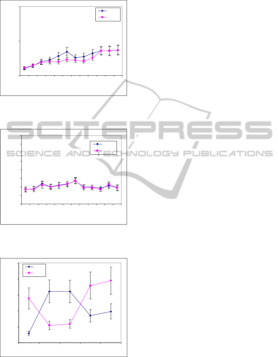
We use Figs. 11 and 12 and Table 5 to plot mean
values ± standard deviation of MSE results as shown
in Figs. 14 and 15. The curves of MSE–ApEn
completely overlap while the MSE–SampEn curves
have only one point (at scale factor 6) which does
not overlap but the separation between two curves at
this point is not good. In this dataset, the application
of MSE is not as good as ovarian cancer data
(section 5.1) because the complexity of this dataset is
higher (the cardiac disease is unclear while the
cancer disease is clarity). For GA–based MSE, we
use Fig. 13 and Table 7 to plot mean values ±
standard deviation as shown in Fig. 16 with a very
high separation and no overlapped points. Therefore,
the separations of curves given by GA–based MSE
are better than MSE.
The above paragraph describes the mean values ±
standard deviation charts to estimate the separation
between two entropy curves. We can also use the
Euclidean distance to evaluate. The distance of MSE
and GA–based MSE is 2.28 while 0.18 and 0.03 are
the distances of MSE–SampEn and MSE–ApEn,
respectively. In this case, the distance of GA–based
MSE is 13 times better than MSE.
Table 5: Standard deviation of MSE analysis of MACE
data.
Scale
factor
SampEn ApEn
Control MACE Control MACE
1 0.0171 0.0191 0.0204 0.0286
2 0.0220 0.0244 0.0201 0.0295
3 0.0355 0.0323 0.0288 0.0400
4 0.0412 0.0345 0.0230 0.0325
5 0.0495 0.0330 0.0253 0.0378
6 0.0624 0.0317 0.0261 0.0320
7 0.0429 0.0297 0.0297 0.0369
8 0.0503 0.0279 0.0229 0.0273
9 0.0541 0.0379 0.0220 0.0274
10 0.0634 0.0530 0.0225 0.0235
11 0.0630 0.0732 0.0342 0.0341
12 0.0644 0.0730 0.0343 0.0275
Table 6: Parameters of GA–based MSE analysis of MACE
data.
M r Scale factor
8 0.0173 5
6 0.0174 6
5 0.0156 7
3 0.0111 9
2 0.0106 12
COMPLEXITY ANALYSIS OF MASS SPECTROMETRY DATA FOR DISEASE CLASSIFICATION USING
GA-BASED MULTISCALE ENTROPY
11
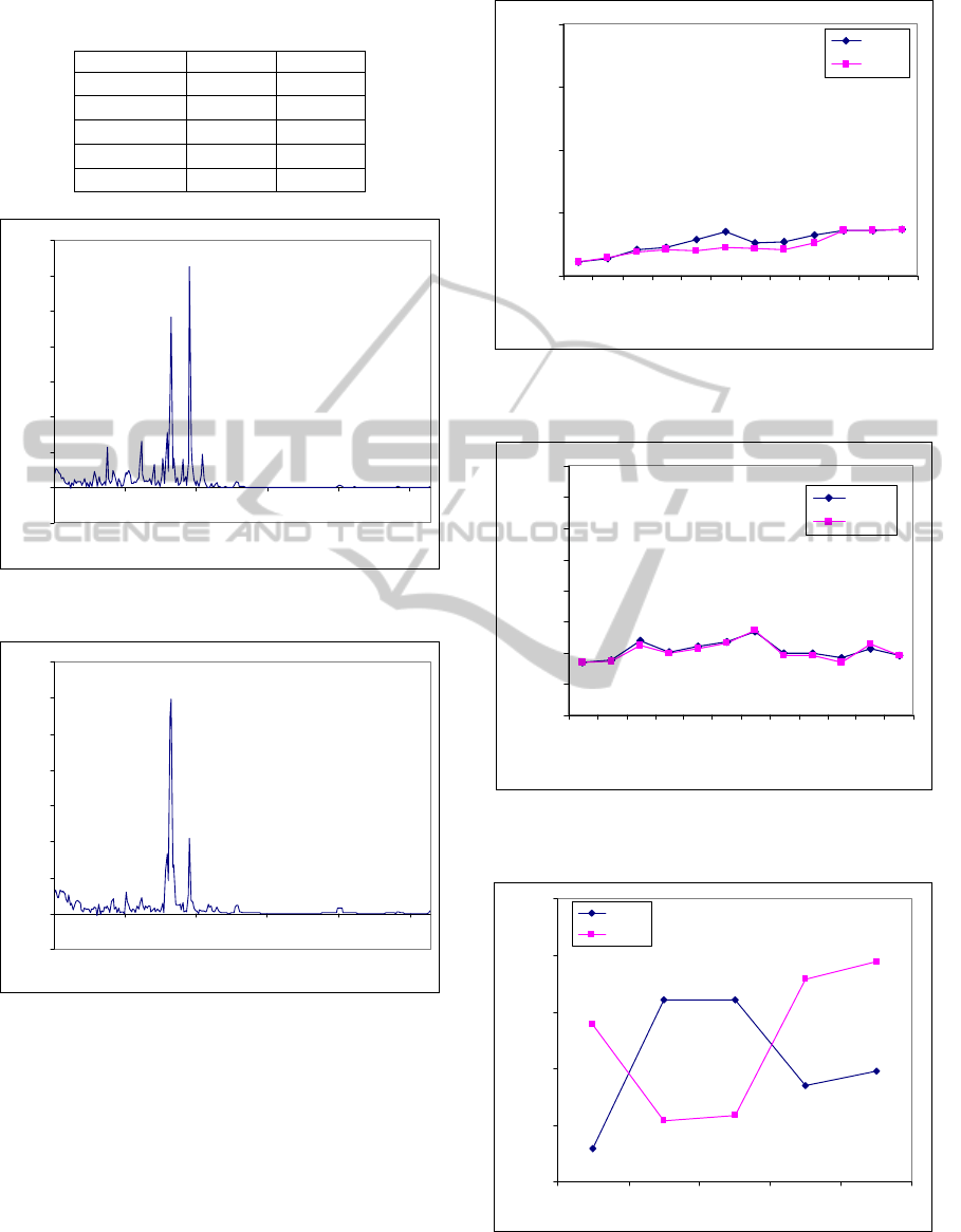
Table 7: Standard deviation of GA–based MSE of MACE
data.
Scale factor Control MACE
5
0.0647 0.3293
6
0.3579 0.1253
7
0.3544 0.1335
9
0.1955 0.4238
12
0.2449 0.4286
-5
0
5
10
15
20
25
30
35
1 51 101 151 201 251
Time index
Relative intensity
Figure 9: SELDI–MS control sample.
-5
0
5
10
15
20
25
30
35
1 51 101 151 201 251
Time index
Relative intensity
Figure 10: SELDI–MS MACE sample.
0
0.5
1
1.5
2
1234 5678 9101112
Scale factor
SampEn
Control
MAC E
Figure 11: MSE–SampEn analysis of MACE dataset
(values are given as means with m = 2, r = 0.02).
0
0.1
0.2
0.3
0.4
0.5
0.6
0.7
0.8
123456789101112
Scale factor
ApEn
Control
MAC E
Figure 12:MSE–ApEn analysis of MACE dataset (values
are given as means with m = 5, r = 0.03).
0
0.5
1
1.5
2
2.5
567912
Scale factor
SampEn
Control
MACE
Figure 13: GA–based MSE analysis of MACE dataset
(values are given as means).
BIOSIGNALS 2011 - International Conference on Bio-inspired Systems and Signal Processing
12
0
0.5
1
1234 5678 9101112
Scale factor
SampEn
Contr ol
MA CE
Figure 14: MSE–SampEn analysis of MACE dataset
(values are given as means ± standard deviation with
m = 2, r = 0.02).
0
0.1
0.2
0.3
0.4
0.5
0.6
0.7
0.8
123456789101112
Scale factor
ApEn
Co nt r ol
MA CE
Figure 15:MSE–ApEn analysis of MACE dataset (values
are given as means ± standard deviation with m = 5,
r = 0.03).
0
0.5
1
1.5
2
2.5
567912
Scale factor
SampEn
Contro l
MA CE
Figure 16: GA–based MSE analysis of MACE dataset
(values are given as means ± standard deviation).
5 CONCLUSIONS
We have introduced the GA–based MSE which is
able to optimally select the control parameters of the
entropy approach to maximize the separation
between the two entropy profiles. The method was
tested against two real mass spectrometry datasets.
The obtained results have shown the effectiveness
the GA–based MSE.
The proposed method can be potentially
improved by using the extended compact GA
(ECGA) (Sastry and Goldberg, 2000) and parallel
GA based on island model (Fernandez, 2005)
(Cantu-Paz, 2001) (Calegari et al., 1997) to enhance
the result and the speed of GA–based MSE. The
crossover operator of classical GA is a random
operator while crossover operator of ECGA is based
on probability model. Therefore, extended compact
GA can be expected to discover appropriate genetic
codes in the population and preserves them for the
next generations. Although each generation of
ECGA takes more time than traditional GA, ECGA
converges to the solution faster than traditional GA.
The results of ECGA are better than classical GA.
The parallel GA based on the island model not only
increases computational speed but also improves the
performance because the island model can exploit all
diversity of population.
ACKNOWLEDGMENTS
This work was supported by under the Australian
Research Council's Discovery Projects funding
scheme (project number DP0877414). The MS data
were provided by Honghui Wang, Clinical Center,
National Institutes of Health, Bethesda, MD 20892,
USA.
REFERENCES
Burioka N., Cornélissen G., et al., 2003. Approximate
entropy of human respiratory movement during eye-
closed waking and different sleep stages. Chest, 123:
80–86.
Burioka N., Cornelissen G., et al., 2005. Approximate
entropy of the electroencephalogram in healthy awake
subjects and absence epilepsy patients. Clin. EEG
Neurosci, 36:188–193.
Caldirola D., Bellodi L., et al., 2004. Approximate Entropy
of Respiratory Patterns in Panic Disorder. Am. J.
Psychiatry, 161:79–87.
COMPLEXITY ANALYSIS OF MASS SPECTROMETRY DATA FOR DISEASE CLASSIFICATION USING
GA-BASED MULTISCALE ENTROPY
13

Calegari P., Guidec F., et al., 1997. Parallel island-based
genetic algorithm for radio network design. Journal of
Parallel and Distributed Computing, 47(1): 86–90.
Cantu-Paz E., 2001. Efficient and accurate parallel genetic
algorithms. Kluwer Academic Publishers.
Castiglioni P. and Di Rienzo M., 2008. How the threshold
“r” influences approximate entropy analysis of heart-
rate variability. Computers in Cardiology, 35:561–564.
Chong K. P. E and Zak H. S., 2001. An Introduction to
Optimization, John Wiley & Sons, New York.
Conrads T. P. and Zhou M., et al, 2003. Cancer diagnosis
using proteomic patterns. Expert Rev. Mol. Diagn., 3:
411–420.
Costa M. and Goldberger A. L., 2002. C.K. Peng,
Multiscale entropy analysis of complex physiologic
time series. Phys. Rev. Lett., 89.
Costa M., Goldberger A. L., Peng C. K., 2005. Multiscale
entropy analysis of biological signals. Phys Rev E Stat
Nonlin Soft Matter Phys., 71.
Costa M., Goldberger A. L., Peng C. K., 2002. Multiscale
entropy to distinguish physiologic and synthetic RR
time series. Computers in Cardiology, 29:137–140.
Eckmann J. P. and Ruelle D., 1985. Ergodic theory of
chaos and strange attractors. Rev. Modern Phys.,
57:617–654.
Eidhammer I., Flikka K., et al., 2007. Computational
methods for mass spectrometry proteomics, Wiley.
Ferenets R., Lipping Tarmo, et al., 2006. Comparison of
entropy and complexity measures for the assessment of
depth of sedation. IEEE Trans. Biomed. Eng.,
53:1067–1077.
Fernandez de Vega F., 2005. Parallel genetic
programming. Workshop 2005 IEEE Congress on
Evolutionary Computation.
Hagan M. T., Demuth H. B., Beale M. H., 1995. Neural
Network Design, PWS Pub. Co..
Ho K. K., Moody G. B., et al., 1997. Predicting survival in
heart failure case and control subjects by use of fully
automated methods for deriving nonlinear and
conventional indices of heart rate dynamics.
Circulation, 96: 842–848.
Hornero R., Aboy M., et al., 2005. Interpretation of
Approximate Entropy: Analysis of Intracranial
Pressure Approximate Entropy During Acute
Intracranial Hypertension. IEEE Trans. Biomed. Eng.,
52:1671–1680.
Kim W. S., Yoon Y. Z., et al., 2005. Nonlinear
characteristics of heart rate time series: influence of
three recumbent positions in patients with mild or
severe coronary artery disease. Physiol. Meas.,
26:517–529.
Koskinen M., Seppanen T., et al., 2006. Monotonicity of
approximate entropy during transition from awareness
to unresponsiveness due to propofol anesthetic
induction. IEEE Trans. Biomed. Eng., 53:669–675.
Lake D. E., Richman J. S., et al., 2002. Sample entropy
analysis of neonatal heart rate variability. Am. J.
Physiol Regul Integr Comp Physiol, 283:789–797.
Lee M-L. T., 2004. Analysis of microarray gene
expression data, Kluwer Academic Publishers, Boston.
Lu S., Chen X., et al., 2008. Automatic selection of the
threshold value r for approximate entropy. IEEE
Trans. Biomed. Eng., 55: 1966–1972.
Mitchell M., 2001. An Introduction to Genetic Algorithm,
MIT Press, London.
Muniyappa R., Sorkin J. D., et al., 2007. Long-term
testosterone supplementation augments overnight
growth hormone secretion in healthy older men. Am. J.
Physiol Endocrinol Metab, 293: 769–775.
Petricoin E. F., Ardekani A. M., et al., 2002. Use of
proteomic patterns in serum to identify ovarian cancer.
The Lancet, 359:572-577.
Pham T. D., Wang H., et al., 2008. Computational
prediction models for early detection of risk of
cardiovascular events using mass spectrometry data.
IEEE Trans.ITB 12:636–643.
Pincus S. M., 1991. Approximate entropy as a measure of
system complexity. Proc. Natl. Acad. Sci. USA, 88:
2297–2301.
Richman J. S. and Moorman J. R., 2000. Physiological
time-series analysis using approximate entropy and
sample entropy. Am. J. Physiol Heart Circ Physiol
278: 2039–2049.
Rukhin A. L., 2000. Approximate entropy for testing
randomness. J. Appl. Probability, 37:88–100.
Sastry K. and Goldberg D. E., 2000. On extended compact
genetic algorithm. GECCO 2000.
Seeger A., 2006. Recent Advances in Optimization,
Springer, Berlin.
To C., Vohradsky J., 2007. A parallel genetic algorithm for
single class pattern classification and its application for
gene expression profiling in streptomyces coelicolor.
BMC Genomics, 8:49.
To C., Vohradsky J., 2007. Binary classification using
parallel genetic algorithm. Proceedings of the 2007
IEEE Congress on Evolutionary Computation, 1281-
1287.
Zhou X., Wang H., et al., 2006. Biomarker discovery for
risk stratification of cardiovascular events using an
improved genetic algorithm. Proceedings of Life
Science Systems and Applications Workshop, 42–44.
BIOSIGNALS 2011 - International Conference on Bio-inspired Systems and Signal Processing
14
