AUTOMATIC SEGMENTATION OF EMBRYONIC HEART IN

TIME-LAPSE FLUORESCENCE MICROSCOPY IMAGE

SEQUENCES

P. Krämer, F. Boto

, D. Wald, F.Bessy, C. Paloc

Vicomtech, Paseo de Mikeletegi 57, 20009 Donostia, San Sebastián, Spain

C. Callol

, A. Letamendia, I. Ibarbia, O. Holgado, J. M. Virto

Biobide, Paseo de Mikeletegi 58, 20009 Donostia, San Sebastián, Spain

Keywords: Segmentation, Fluorescent microscopy images, Embryonic heart.

Abstract: Embryos of animal models are becoming widely used to study cardiac development and genetics. However,

the analysis of the embryonic heart is still mostly done manually. This is a very laborious and expensive

task as each embryo has to be inspected visually by a biologist. We therefore propose to automatically

segment the embryonic heart from high-speed fluorescence microscopy image sequences, allowing

morphological and functional quantitative features of cardiac activity to be extracted. Several methods are

presented and compared within a large range of images, varying in quality, acquisition parameters, and

embryos position. Although manual control and visual assessment would still be necessary, the best of our

methods has the potential to drastically reduce biologist workload by automating manual segmentation.

1 INTRODUCTION

Model organisms have become more and more

important for the study of vertebrate development.

Due to its prolific reproduction and the external

development of the transparent embryo, they are

prime models for genetic and developmental studies,

as well as research in toxicology and genomics.

While genetically more distant from humans, the

vertebrate models nevertheless have comparable

organs and tissues, such as heart, kidney, pancreas,

bones, and cartilage.

During the last years tremendous advances in

imaging system have been made allowing the

acquisition of high-resolution images of embryos.

Anyhow, the processing of such images is still a

challenge (Vermot et al., 2008). To date, only little

work has been presented addressing the analysis of

embryo models images (Fink et al., 2009; Luengo-

Oroz et al., 2007; Liebling et al., 2006). For instance

(Liebling et al., 2006) presents a method to acquire,

reconstruct and analyze 3D images of the zebrafish

heart. The reconstruction of the volume is based on a

semi-automatic segmentation procedure and requires

the help of the user. Fink et al., 2009 propose a

method for detection and quantification of heartbeat

parameters in Drosophilia deriving a signal from the

images, avoiding segmentation.

In case of studies of cardiac development, a

segmentation of the heart provides additional

information for its quantification. Therefore, we

present several approaches to automatically extract

its shape and each chamber from image sequence. In

our experiment, transgenic embryos expressing

fluorescent protein in the myocardium were placed

under light microscopy allowing to capture

fluorescent images of the heart at video rate. In

particular, we are interested in segmenting the heart

of zebrafish embryos after two days of post-

fertilization (2 dpf). In early stages of the zebrafish

development the primitive heart begins a simple

linear tube. This structure gradually forms into two

chambers, a ventricle and an atrium. At 2 dpf the

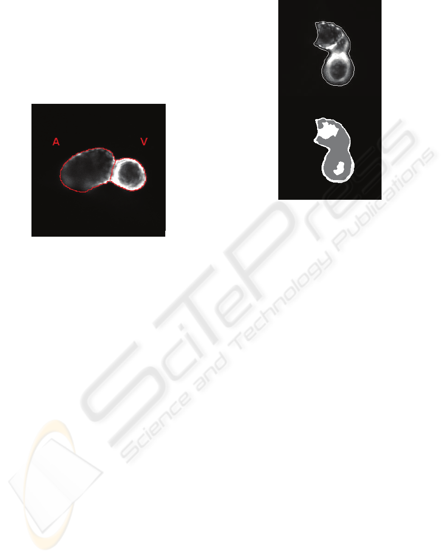
heart tube is already partitioned into atrium and

ventricle as depicted in Figure 1. They are separated

by a constriction which will later form the valve. At

this stage the heart is already beating. More

information on zebrafish heart anatomy can be found

121

Krämer P., Boto F., Wald D., Bessy F., Paloc C., Callol C., Letamendia A., Ibarbia I., Holgado O. and Virto J. (2010).

AUTOMATIC SEGMENTATION OF EMBRYONIC HEART IN TIME-LAPSE FLUORESCENCE MICROSCOPY IMAGE SEQUENCES.

In Proceedings of the Third International Conference on Bio-inspired Systems and Signal Processing, pages 121-126

DOI: 10.5220/0002342501210126

 SciTePress

in (Hu et al., 2000).

The remainder is organized as follows: In section

2 we present several approaches to segment the

zebrafish heart and in section 3 two methods to

identify the chambers. In section 4 we show some

results and compare the segmentation methods

respectively for the heart and its chambers. We give

a conclusion of our work and outline future research

in section 5.

Figure 1: The 2 dpf zebrafish heart already consists of two

chambers: the atrium (A) and ventricle (V).

2 SEGMENTATION OF THE

ZEBRAFISH HEART

In this section we outline different approaches to

segment the shape of the zebrafish heart. For the

methods of subsection 2.3, 2.4, 2.5, we cast the

images to 8-bit grey level images and stretch the

grey level range into [0,255].

2.1 Adaptive Binarization

This method is based on the assumption that the

image of the heart consists of three brightness levels

such as illustrated in Figure 2: one corresponding to

the background and two corresponding to the

fluorescent heart where strong contracted regions

appear brighter due to a higher concentration of

fluorescent cells.

For pre-processing, we smooth image using a

Gaussian filter to remove noise. Then, the region of

the heart with highest brightness is segmented by

first applying a Contrast-Limited Adaptive

Histogram Equalization (CLAHE) (Zuiderveld,

1994) using a uniform transfer function and then the

automatic threshold method from Otsu (Otsu, 1979).

In order to segment the second, less brighter region

of the heart, we exclude the previous segmented

Figure 2: The image of fluorescent heart consists of three

brightness levels: one corresponding to the background

and two to the heart.

region and apply CLAHE and Otsu again. The

final segmentation is obtained by combining both

segmentation results. Postprocessing includes the

filling of holes which can appear inside in the shape.

2.2 Clustering

This method is based on unsupervised classification

in order to distinguish between object and

background pixels. First, each pixel is characterized

by the mean luminance value of the 3×3 mask

centered at the pixel. A unidimensional feature space

results. Then, we use a k-means classifier (k=3) in

order to separate the pixels into three clusters. This

method relies like the previous one on the

assumption than that there are three different

brightness levels. The cluster to which belongs the

pixel at position (0,0) is then defined as the

background and others as the region of the heart.

Similarly than above, we apply hole filling as

postprocessing. For more information on k-means

clustering can be found in (Bishop, 2007).

2.3 Voronoi-based Segmentation

The Voronoi segmentation (Imelinska et al., 0002) is

based on repeatedly dividing an image into regions

using Voronoi diagram and classifying the regions

as either inside or outside the target based on

classification statistics, and then break up the

regions on the boundary between the two

classifications into smaller regions and repeat the

BIOSIGNALS 2010 - International Conference on Bio-inspired Systems and Signal Processing

122

classification and subdivision on the new set of

regions. The classification statistics can be obtained

from an image prior which is a binary image of

preliminary segmentation.

In order to compute the image prior, we apply

first a bilateral filter to smooth the image while

preserving edges. Afterwards, the gradient

magnitude is computed using a recursive Gaussian

filter and Sigmoid filter to map the intensity range

into [0,255]. Then a threshold is applied to the

gradient magnitude to obtain a binary mask. As the

binary mask may contain holes, we apply a

morphological closing operation and fill the holes to

complete the object’s shape. Then the main region of

the heart is isolated from noise in the binary image

by a region growing algorithm to the binary with the

brightest pixel in the image as seed point. Typically,

the brightest pixel in the gray-level image belongs to

the region of the heart. After the Voronoi

segmentation we apply again morphological closing,

hole filling, isolation of the main region, and

morphological erosion to smooth the contours.

2.4 Level Set

The idea of this method is similar to the previous

one. First a pre-segmentation accomplished which is

then refined, but here we use the level set approach

(Li et al., 2005) for refinement. We choose this

method because of its fast performance.

The method starts with a morphological

reconstruction to suppress structures that are lighter

than their surroundings and that are connected to the

image border. Then, edges are detected using the

Canny edge detector. Dilation, hole filling, and

erosion are applied to the contour image. The

biggest region is considered as the region of the

heart while the others are considered as noise. We

complete the form by applying again dilation and

hole filling.

A Gaussian filter is applied to smooth the

original grey level image for noise removal. Then

we apply the level set method (Li et al., 2005) with

contours of the binary mask as initialization. We

chose the edge indicator function 1/(1+g) as

suggested by the author where g is the gradient

magnitude of the Gaussian filtered grey level image.

2.5 Watershed

This approach is different to the previous one as it

does not rely on a pre-segmentation by binarization.

It is based on Watershed segmentation.

First the border structures are supressed by

morphological reconstruction. This is followed by a

strong low-pass filtering (Gaussian filter) in a

morphological reconstruction by erosion using the

inverse of morphological gradient. This attenuates

unwanted portions of the signal while maintaining

the signal intensity as the Watershed method is

known to oversegment the image. Afterwards, a

small threshold is applied to set the background to

zero and the image intensity is adjusted so that such

that 1% of data is saturated at low and high

intensities. We apply to this gradient magnitude the

watershed segmentation. An oversegmented image

may result with typically one region belonging to the

background and several regions belonging to the

heart. The latter ones are joined to form the region of

the heart.

3 IDENTIFICATION OF THE

CHAMBERS

The objective is now to divide the heart into the

chambers based on the results of the methods

presented in the previous section.

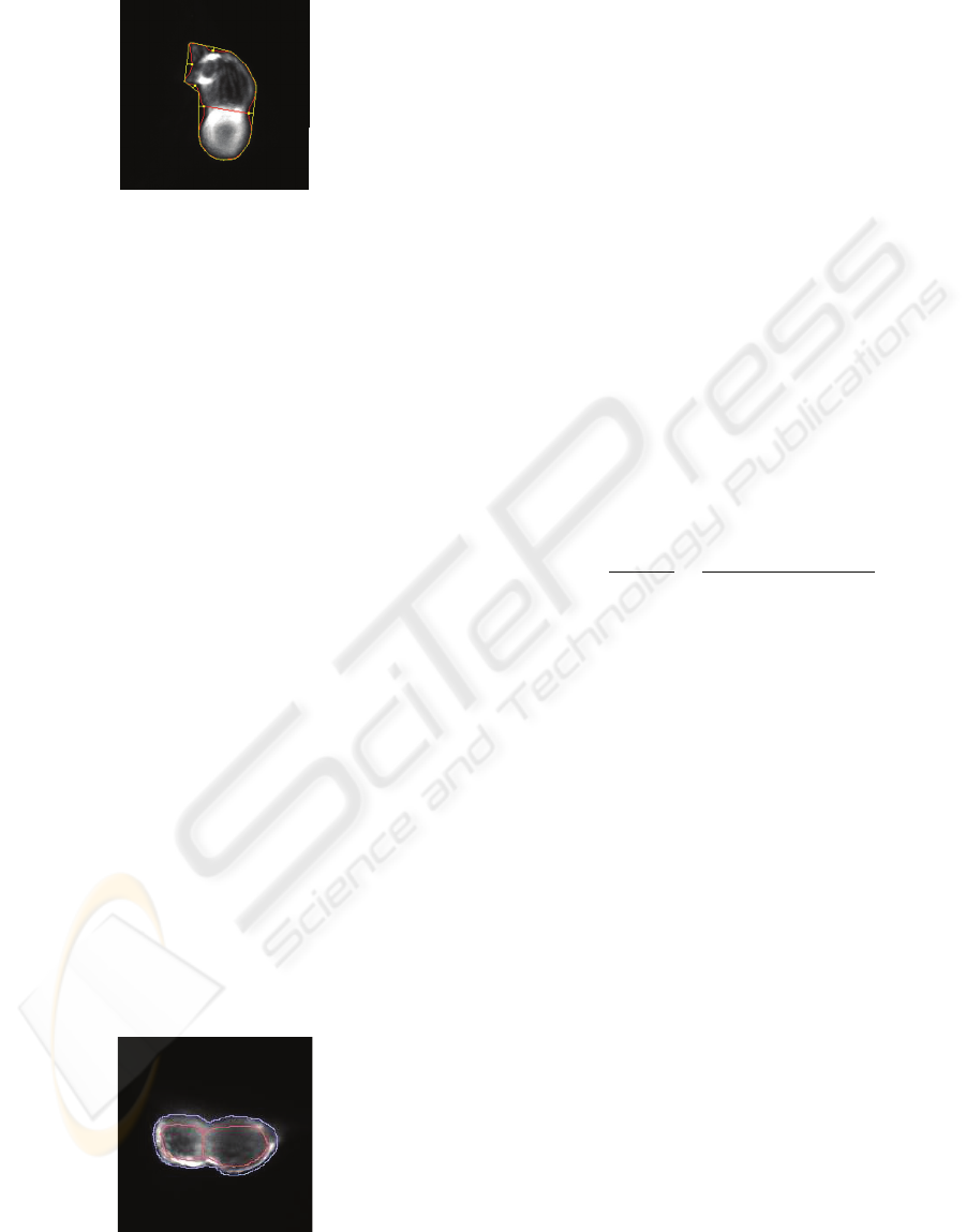
3.1 Convexity Defects

The method assumes that there is a constriction

between the two chambers (see Figure 1) causing

two convex points in the contour of the heart’s

shape. Therefore, we compute the convexity defects

of the contour using its convex hull. Generally more

than two convexity defects are found due to

irregularities in the contour caused by the

segmentation as depicted in Figure 3. Moreover, we

assume that the convexity defects denoting the

constriction between the chambers are parallel.

Thus, we choose the four most important convexity

defects, i.e. the four points with the highest distance

from the convex hull, and compute the angle for

each pair as:

  















(1)

where v1,v2 are respectively the vectors between the

start and end points of the first and second convexity

defects. If the angle is lower than a small threshold,

then the pair of convexity defects is considered as a

possible candidate for the constriction, otherwise it

is rejected. Finally, we choose the pair with the

highest mean distance as the points of the

constriction from the remaining. We compute the

straight line interpolating the points which separates

both chambers. As there is often a high variation of

the straight line along the image sequence, we

correct it by Double Exponential Smoothing-Based

AUTOMATIC SEGMENTATION OF EMBRYONIC HEART IN TIME-LAPSE FLUORESCENCE MICROSCOPY

IMAGE SEQUENCES

123

Prediction (DESP) (LaViola Jr., 2003) using the

results of the previous images.

Figure 3: The segmented heart (inside line) and the convex

hull (outside line) with convexity defects of the shape

(points).

3.2 Watershed

This method is based on the results of the Watershed

segmentation of subsection 2.5. The general idea is

to divide the segmented shape into the two chambers

by applying a second watershed segmentation.

Therefore, the background is masked out and a

watershed segmentation is applied in this area after a

strong low-pass filtering. If two regions result, then

they correspond to a rough identification of two

chambers. Otherwise the regions have to be joined

until only two regions remain. Therefore, we use the

chamber identification of the previous image. We

compute the intersection of a region in the current

image with the identified chambers of the previous

image. Then, the region is identified to belong to the

chamber where the intersection is maximal. It can

happen that only one region is obtained by the

Watershed segmentation. Then, the segmentation of

the previous image is used for further processing of

the current image.

This chamber identification is very rough

whereas the outline is not coincident with that one of

subsection 2.5 as can be seen in Figure 4. Thus

unassigned pixels remain. In order to assign them to

one of the chambers, an Euclidean distance

transform is computed for each chamber. Then, the

non-assigned pixels of the segmentation are joined

with the chamber for which the distance transform is

smaller.

Figure 4: The Watershed segmentation (outline line) and

the first rough identification of the chambers (inside line).

4 RESULTS AND DISCUSSION

In this section, we show and discuss the results

obtained with the methods presented above. First,

we compare the algorithms for segmenting the shape

of the heart from section 2 using an accuracy

measure. Then, we evaluate visually the results of

chamber segmentation algorithms from section 3.

4.1 Comparison of Segmentation

Algorithms

Several methods exist to measure the performance of

segmentation algorithms (Zhang et al., 2008; Sezgin

and Sankur, 2004). Here, we choose to compare the

segmented images with ground truth images which

were obtained by manual segmentation.

We used the Jaccard coefficient (Cox and Cox,

2001; Ge et al., 2007) as performance measure for

each segmentation method. This coefficient

measures the coincidence between the segmentation

result R and the ground truth A. Then, the

segmentation accuracy is measured as:





,

































(2)

with

as the number of pixels of the given region.

The nominator



means how much of the

object has been detected while the denominator



is a normalization factor to scale the

accuracy measure into the range of [0,1]. Likewise

pixels falsely detected as belonging to the object

(false positives) are penalized by the normalization

factor. Thus, this accuracy measure is insensitive to

small variations in the ground truth construction and

incorporates both, false positives and negatives, in

one unified function (Ge et al., 2007).

In our experiments we used 26 image sequences

with a resolution of 124×124 pixels. For each image

sequence we segmented the first 20 images with the

above presented methods and compared them with a

ground truth segmentation. We only chose

sequences with fair image quality for evaluation as

otherwise the accuracy of the manual segmentation

is too subjective (Figure 5).

The results of Jaccard coefficient for each sequence

are presented in Table 1. The Voronoi-based and

both thresholding methods outperform the watershed

and level set methods. A visual inspection of the

segmentation results reveals similar results.

BIOSIGNALS 2010 - International Conference on Bio-inspired Systems and Signal Processing

124

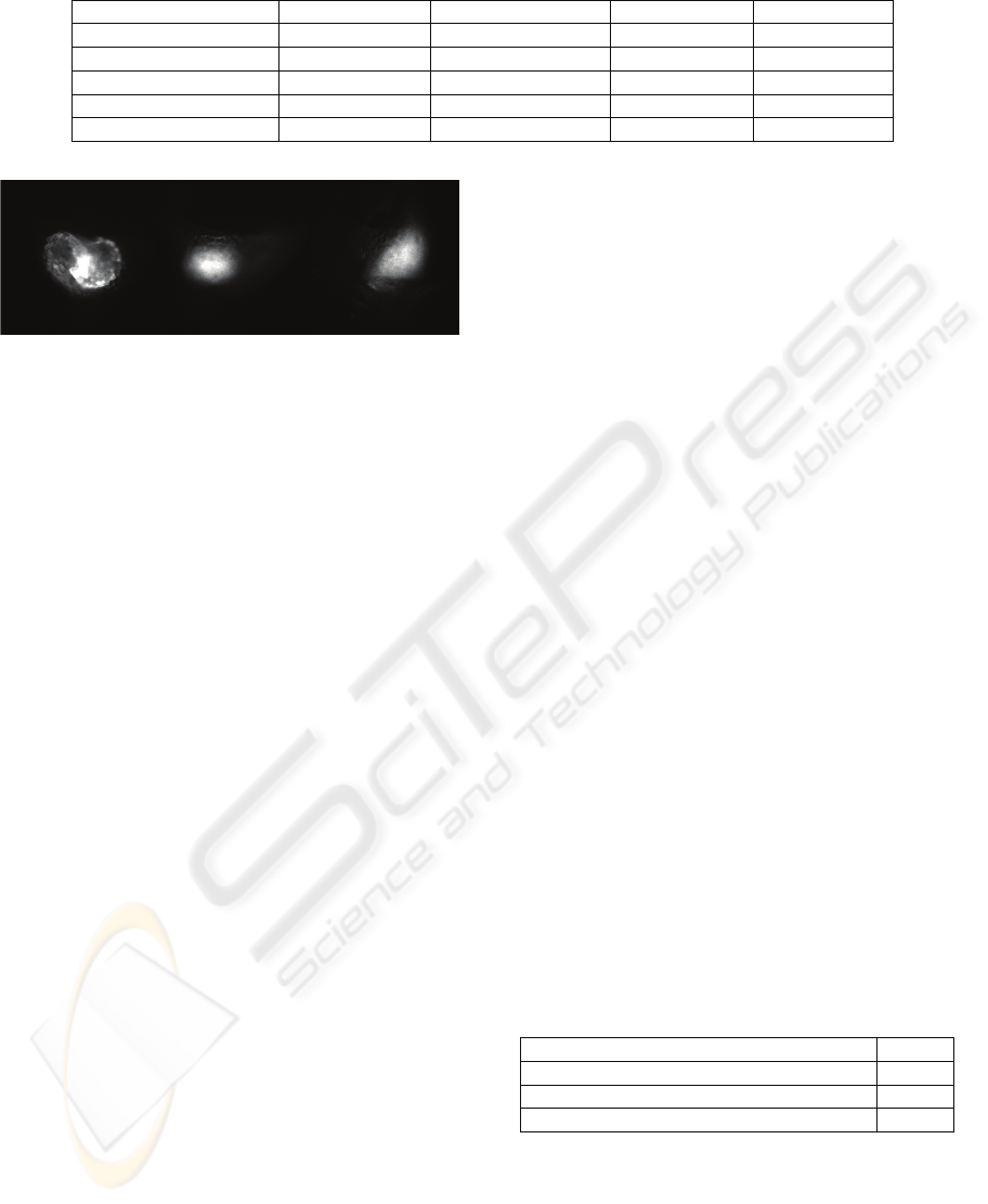
Table 1: Mean accuracy for the segmentation algorithms.

Method Mean accuracy Standard deviation Max accuracy Min accuracy

Adaptive binarization 0.870 0.052 0.946 0.725

Clustering 0.876 0.057 0.954 0.759

Voronoi segmentation 0.890 0.046 0.937 0.769

Level set 0.850 0.062 0.965 0.724

Watershed 0.856 0.044 0.896 0.717

Figure 5: Rejected samples. Overlapping chambers and

blurred images.

The level set method gives good results on high

contrast edges, but in regions where edges are

blurred, the level set does not approach well the

shape of the heart resulting in holes in the object

shape or a too large shape. Moreover, we found it

difficult to determine a common set of parameters

suitable for all sequences.

The contours of the watershed method appear

very rough and are often too tight. This might be due

to the strong low-pass filtering in the post-

processing which causes an edge mismatch. Equally

a false classification of the regions into background

and foreground may cause an inaccurate

segmentation.

The Voronoi-based segmentation method reveals

the best results in term of accuracy measure. The

contours are typically slightly irregular; some

postprocessing could be applied to smooth them. In

case of low-contrast contours it may behave similar

to the level set method. The overall results are quite

satisfying.

The adaptive binarization tends to have a slightly

larger contour, but approaches well the object shape.

This might cause the lower accuracy results, but the

overall segmentation results are good. Sometimes in

case of low-contrast edges the object shape may be

incomplete.

The clustering method tends also to larger

contours, but slightly tighter than the adaptive

binarization method. Therefore, a higher accuracy is

achieved. However, in case of low-contrast edges it

reveals more often incomplete shapes than the

adaptive binarization. Note that the accuracy can

vary as the randomized choice of initial cluster may

result in slightly different segmentation results.

The computational cost cannot be directly

compared as the implementations use different

programming languages and libraries (the adaptive

binarization, clustering, and Voronoi methods are

implemented in C++ using respectively OpenCV,

OpenCV and Torch, and ITK; the level set and

watershed methods are implemented in Matlab).

However, the execution time for each image is

reasonable and estimated at about one second

independently of the method.

4.2 Chamber Identification

In this section, we present some results of the

convexity defects and watershed methods used to

divide the heart into two chambers. The convexity

defects method was evaluated only in combination

with the adaptive binarization and clustering

methods, as they present good segmentation results

(see previous section).

For evaluation we used only 24 out of the 26

sequences from above, because in two other ones the

chambers are superimposed (Figure 5). Such cases

are not taken in consideration in current

developments, and we therefore chose to discard

those sequences. 480 images were then segmented

using each of the described method, and visually

inspected to evaluate whether the heart was correctly

divided. Our results are shown in Table 2, where the

best result is obtained for the adaptive binarization

method.

Table 2: The ratio of correct chamber identification per

image for the chamber identification algorithms.

Method Ratio

Adaptive binarization + convexitydefects 0.704

Clustering + convexity defects 0.577

Watershed 0.456

5 CONCLUSIONS AND FUTURE

WORK

We presented a first attempt of automatically

segmenting the shape and the chambers of the

AUTOMATIC SEGMENTATION OF EMBRYONIC HEART IN TIME-LAPSE FLUORESCENCE MICROSCOPY

IMAGE SEQUENCES

125

zebrafish embryonic heart from time-lapse

fluorescence microscopy image sequences.

For segmenting the shape of the heart, the

Voronoi-based and both thresholding methods

outperform the watershed and level set methods. The

Voronoi-based segmentation gives the best results in

terms of the accuracy measure, as thresholding

methods tend to fail in cases of low-contrast edges.

The watershed segmentation results in quite

rough contours. Anyhow, it is an interesting

approach as it is the basis for chamber identification.

The results of the level set method are not satisfying.

For chamber identification the adaptive binarization

method in combination with the detection of

convexity defects outperforms clearly the other

methods.

Besides segmentation in order to extract

morphological information, we are also working on

other processing methods to extract cardiac function

metrics from image sequence. Such methods are

able to provide additional information for cardiac

development study with very high accuracy.

REFERENCES

Bishop, C.M. (2007). Pattern Recognition and Machine

Learning. (Information Science and Statistics).

Springer.

Cox, T. and Cox, M. (2001). Multidimensional Scaling

(2nd ed.). Chapman & Hall/CRC.

Fink, M., Callol-Massot, C., Chu, A., Ruiz-Lozano, P.,

Belmonte, J. C., Giles, W., Bodmer, R., and Ocorr, K.

(2009). A new method for detection and quantification

of heartbeat parameters in drosophila, zebrafish, and

embryonic mouse hearts. BioTechniques, 46(2), 101–

113.

Ge, F., Wang, S., and Liu, T. (2007). New benchmark for

image segmentation evaluation. Journal of Electronic

Imaging, 16(3):033011.

Hu, N., Sedmera, D., Yost, H., and Clark, E. (2000).

Structure and function of the developing zebrafish

heart. The Anatomical Record, 260(2), 148–157.

Imelinska, C., Downes, M., and Yuan, W. (2002). Semi-

automated color segmentation of anatomical tissue.

Computerized Medical Imaging and Graphics, 24,

173–180.

LaViola Jr., J. (2003). Double exponential smoothing: An

alternative to kalman filter-based predictive tracking.

In Immersive Projection Technology and Virtual

Environments, 199–206.

Li, C., Xu, C., Gui, C., and Fox, M. (2005). Level set

evolution without re-initialization: A new variational

formulation. CVPR, 1, 430–436. IEEE.

Liebling, M., Forouhar, A., Wolleschensky, R.,

Zimmermann, B., Ankerhold, R., Fraser, S., Gharib,

M., and Dickinson, M. E. (2006). Rapid three-

dimensional imaging and analysis of the beating

embryonic heart reveals functional changes during

development. Developmental Dynamics, 235(11),

2940–2948.

Luengo-Oroz, M., Faure, E., Lombardot, B., Sance, R.,

Bourgine, P., Peyri´eras, N., and Santos, A. (2007).

Twister segment morphological filtering. A new

method for live zebrafish embryos confocal images

processing. ICIP, 253–256. IEEE.

Otsu, N. (1979). A threshold selection method from

graylevel histograms. IEEE Trans. on Systems, Man

and Cybernetics, 1(9), 62–69.

Sezgin, M. and Sankur, B. (2004). Survey over image

thresholding techniques and quantitative performance

evaluation. Journal of Electronic Imaging, 13(1), 146–

168.

Vermot, J., Fraser, S., and Liebling, M. (2008). Fast

fluorescence microscopy for imaging the dynamics of

embryonic development. HFSP Journal, 2(3), 143–

155.

Zhang, H., Fritts, J., and Goldman, S. (2008). Image

segmentation evaluation: A survey of unsupervised

methods. Computer Vision and Image Understanding,

110(2), 260–280.

Zuiderveld, K. (1994). Graphics Gems IV, chapter

Contrast Limited Adaptive Histogram Equalization,

pages 474–485. Academic Press.

BIOSIGNALS 2010 - International Conference on Bio-inspired Systems and Signal Processing

126