DETECTION OF A FAULT BY SPC AND IDENTIFICATION
A Method for Detecting Faults of a Process Controlled by SPC
Massimo Donnoli
DSEA – Dept. Electrical Systems and Automation, University of Pisa, Italy
Keywords: Statistical process control, Multivariate Hotelling statistic, System identification.
Abstract: A method for detecting the nature of a fault of a process controlled by SPC ( Statistical Process Control) is
presented. The method use the integration of SPC , traditional APC (Automatic Process Control) and the
System Identification technique . By a statistical on line control of the parameters of a transfer function and
the identification of the transfer function itself, the case of a fault due to a change in the system is
recognised. An algorithm called ‘batch control’ for the implementation of the method in a real plant is
proposed.
1 INTRODUCTION
The objective of Statistical Process Control (SPC) is
to detect situation of change of the natural behaviour
of a process by monitoring on line the key product
variables and detecting the cause of the fault,
indicating which variable or group of variables
contributes to the signal.
A lot of technique has been developed especially
due to the large and different areas where the SPC
could be applied.
If, traditionally, the SPC has been developed
especially to monitor the complicated processes of
chemical plants, after that, the big growth of the
information technology in the industries and the
large amount of process measures collected in the
data base of the control systems, has allowed the
implementation of SPC on almost every kind of
plant. By the way the common goal for the most
application is still to monitor the quality of the
process, treating the manufacturing process itself as
a black box, of which we know the inputs and
outputs, ignoring the others information of the
nature of the process.
In fact traditionally SPC and APC (Automatic
Process Control) have been developed in parallel
and only in the last years there has been works
where researchers have made the integration of the
two areas ( Tsung,1999).
Another point to remark is that the traditional
SPC approach, that is still the most diffused in many
kind of industries, is essentially the univariable SPC:
by the implementation of control charts like
Shewhart, Cusum, etc.. we look the magnitude of the
deviation of each variable independently of all
others as they are perfectly independent in the
process.
But the being ‘in control’ of a process is
essentially a multivariable property : in the modern
industrial processes the variables are non
independent of one another and only if the
simultaneous state of them all is in the joint
confidence region defined for the system, we could
say that the system is in control : by examining one
variable at time with the traditional charts it could
be that every variable is in the correct range but the
common state is not (Kourti & MacGregor,1994).
For this have been developed multivariable
methods that can treat all the variables
simultaneously.
The principal is the Hotelling or
2
T
statistic : it
transforms the state of all the variables in the
calculation of the value of a single variable which
can be monitor for detecting faults.
If this is a great effort to solve the problem in a
very useful way, on the other hand we have now the
problem to detect the cause of the fault, the variable
responsible.
This paper is organized as follows: in the next
section the basic concepts of SPC multivariable, the
Hotelling statistic and the interpretation of a
2
T
value are recalled. In sections 3 and 4 the main
advantages of SPC - APC integration and SPC -
System Identification integration are presented.
371
Donnoli M. (2009).
DETECTION OF A FAULT BY SPC AND IDENTIFICATION - A Method for Detecting Faults of a Process Controlled by SPC.
In Proceedings of the 6th International Conference on Informatics in Control, Automation and Robotics - Intelligent Control Systems and Optimization,
pages 371-375
DOI: 10.5220/0002203603710375
Copyright
c
 SciTePress

In section 5 a method for statistically monitoring
the points of a system transfer function is presented.
In section 6 are given the simulation results for a
typical industrial APC. In section 7 an algorithm
called ‘batch control’ for the implementation of the
technique in some kind of industrial processes is
presented . Finally some conclusions are given.
2 SPC MULTIVARIABLE
Suppose that our process has 2 measures represented
by 2 random variables x1,x2 uncorrelated, with
mean value
2,1
μ
μ
and variances
2,1
σ
σ
respectively. Consider the distance of an observation
point from the mean point in the plane (x1,x2).
Instead of the usual Euclidean distance we consider
the relationship :
2
2
2
2
2
)(
2
)22(
1
)11(
SD
XX
=
−
+
−
σ
μ
σ
μ
(1)
This is called ‘statistical distance’ (SD) . For an
observation the contribution of each coordinate to
determining the distance is weighted inversely by its
standard deviation, that means that a change in a
variable with a small standard deviation will
contribute more to the statistical distance than a
change in a variable with a large standard deviation.
It follows that the statistical distance is a measure of
the respect of the statistical behaviour of the two
variables.
If they are correlated it will be an additional term
in x1 x2 and in the plane the curve with constant SD
will be an ellipse, eventually tilted according to the
correlation sign.
In general if we have a process of p variables
and we have n observation vector of the p variables
with the system ‘in control’ (or what is called the
Historical Data Set (HDS) of the system) we can
calculate an estimation of the main vector and of the
covariance matrix of the random variables :
X1
X2
1
μ
2
μ
0
12
=
σ
0
12
>
σ
0
12
<
σ
Figure 1: Curves with constant SD for two variables.
∑
=
=
n
i
i
X
n
1
1
μ
(2)
⎥
⎥
⎥
⎥
⎦
⎤
⎢
⎢
⎢
⎢
⎣
⎡
=∑
pppp
p
p
σσσ
σσσ
σσσ
"
#"##
"
"
21
22221
11211
(3)
For a generic observation we can then compute
the quantity :
)()(
12
μμ −∑−=
−
i
T
i
XXT
(4)
This is an univariate quantity that is called
Hotelling Statistic or
2
T
. It is clear that this is the
multivariable generalization of the statistic distance,
in words a measure of the closeness (in a statistical
way) of the observation to the behaviour of the
system expressed by the HDS .
The curves with constant
2
T
are then hyper-
ellipsoids in the p dimensional space.
Considering
2
T
like a random variable we can
see that , in the case of
μ
and
∑
estimate by the
observations, it follows the distribution of an F
random variable of p, n-p degrees of freedom.
Let
α
be the first type error and let
),,( pnp
F
− α
be the value f of F | P(F<=f) = 1-
α
( P : probability
of) we can then calculate an Upper Control Limit
(UCL) for
2
T
:
),,(
)(
)1)(1(
pnp
F
pnn
nnp
UCL
−
−
−
+
=
α
(5)
We can say that if we are under the UCL we
have a probability 1-
α
to say that the system is in
control when really it is .We can see that choosing
an
α
smaller led to have a second type error
β
bigger, that is a greater probability to not detect a
fault when it really exists.
In the industrial processes both errors are
important:
α
is the representation of the false alarms
that can led to stop the production in vain, while
β
,
if large, can led to not detect situations of real out of
control.
Generally
β
is set low because is preferable to
have some false alarm than to not detect a fault .
In our examples we have chosen
α
= 0.1.
2.1 Interpretation of
2
T
Signals
The
2
T
converts a multivariable problem to the
calculation of an univariate quantity. But signal
interpretation requires a procedure for isolating the
responsible of the fault because the contribution
could be attributed to individual variables being
ICINCO 2009 - 6th International Conference on Informatics in Control, Automation and Robotics
372

outside their allowable range of operation or to a
fouled relationship between two or more variables.
Several solutions have been presented for the
problem of interpreting a multivariate signal.
One that we show here for example is the MYT
decomposition (Mason –Young 2002), that uses an
orthogonal transformation to express the
2
T
values
as two orthogonal equally weighted terms :
2
1,2
2
1
2
TTT +=
(6)
2
1
2
11
2
1
/)( σ xxT −=
(7)
2
1,2
2
1,22
2
1,2
/)( σ xxT −=
(8)
where x2,1 is the estimate of the conditional main of
x2 for a given value of x1 and
1,2
σ
is the
corresponding estimate of the conditional variance
of x2 for a given value of x1. A large value of the
first term (called ‘unconditional term’) implies that
the observed value of the variable is outside his
operational range as was on HDS, while a large
values of the second term (‘conditional term’)
implies that the observed value of one variable is not
where it should be relative to the observed value of
the others variables.
By subsequently eliminations of the
unconditional terms that signal and iterative
decomposition of the conditional terms that signal, it
is possible to isolate the variable or group of
variables responsible of the fault. We can say that
all this methods have in common iterative
procedures and sometimes great computational
efforts to reach the scope.
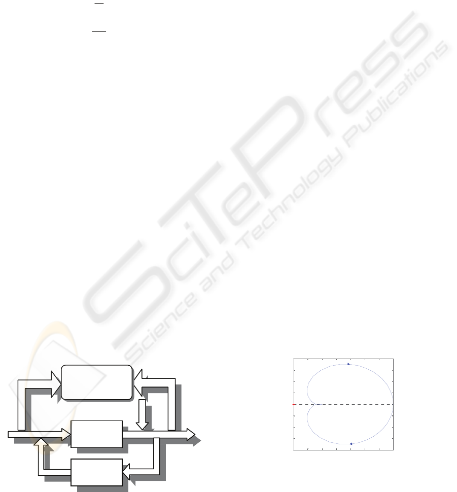
3 SPC APC INTEGRATION
Combining SPC with APC could be an improvement
of the global control of the system.
The scheme is the following :
Figure 2: SPC - APC integration.
There is an interaction between SPC and APC :
SPC controls not only the variables in and out of the
process but also the signals of the control: the result
is that the process is no more treated like a black box
but the information in the APC are used.
Our procedure uses the information of the
transfer function of the system: the change of the
system is statistically monitored controlling the
parameters of the transfer function
4 SPC – SYSTEM
IDENTIFICATION
An industrial system is typically formed by
automation systems that process the product .
We can divide the entire set of variables of the
manufacturing process into ‘process variables’,
meaning that they are measures made above the
product, (temperature, time of operations etc) and
‘control variables’ (like input - output of the motors,
signals of the electronic devices , etc.. ) that reflect
the behaviour of the automation systems.
We propose the identification of the transfer
functions of the control systems and the statistical
monitoring of the transfer functions to detect
deviation of the automation system from their
normal behaviour .
The identification at the same time allow a better
design of the control and a more easily detection of
the fault due to the automation systems and not to
the process .
5 STATISTICAL CONTROL OF A
TRANSFER FUNCTION
Consider the simple transfer function of a system G:
-1 -0.5 0 0.5 1 1.5 2 2.5
-2
-1.5
-1
-0.5
0
0.5
1
1.5
2
Nyquist Diagr am
Real Ax i s
Imaginary Axis
Figure 3: Nyquist plot of a transfer function G.
We can consider the transfer function as a
function of 3 parameters : amplitude, phase and
Process
Control
SPC
DETECTION OF A FAULT BY SPC AND IDENTIFICATION - A Method for Detecting Faults of a Process Controlled
by SPC
373

frequency. So we can plot the function in the 3d
space of that measures :
-1
0
1
2
-200
-150
-100
10
15
20
25
30
Mod
Fase
Freq
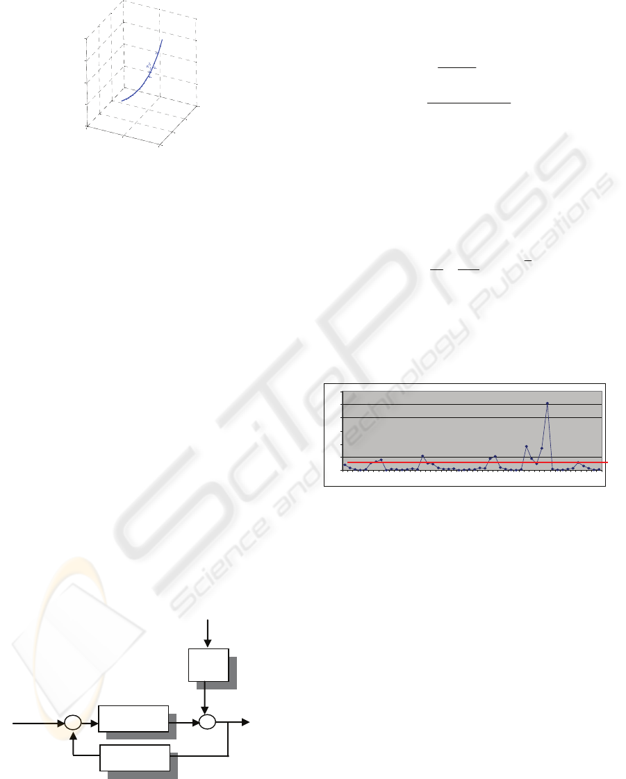
Figure 4: Observations of G points in the space
amplitude-phase-frequency.
If we can do measurements of that parameters our
observations will be point around the real curve of
the transfer function as shown above.
If we plot the curve at constant statistical
distance they will be ellipsoid in the 3d space with
their major axis tangent at the curve of the G in the
point we are sampling it. That tangent is the best
linear approximation of the population, because the
variables follow the relationship of the G.
So we have that schema for the identification
and statistic control of the G:
Make an HDS by collecting observations of the
points of the transfer function while the system is in
his normal behaviour.
Estimate from the HDS the covariance matrix
and the average value of the observations (2) (3).
Set an UCL for the Hotelling statistic chosen a
desired
α
(5).
Monitoring the T2 control chart build with (4).
6 SIMULATION RESULTS
We present the simulation result of a typical
industrial APC :
G(z)
C(z)
D(z)
u(t)
y(t)
d
a(t)
x(t)
Figure 5: Model for simulations.
formed by a system controlled by a PID controller
and disturbed with a coloured noise in the output,
according to the typical modelling of an industrial
noise.
))1()(()()()(
0
−−−−−−=
∑
∞
=
tytykjtyktyktx
D
j
IP
tt
a
Z
Z
D
1
1
1
1
−
−
−
−
=
φ
θ
32.02,1
9.0
)(
2
+−
=
zz
z
zG
),0(
at
Na
σ
∈
(9)
For the on line measurement of the point of the G
we have used the technique of the Descriptive
Function by inserting a relay with hysteresis h and
amplitude A in the control loop.
Leading the system in a controlled oscillation we
can see that the relationship
)(
4
1
)(
c
Y
h
arcsenj
c
c
e
A
Y
F
G
+−
=−=
π
π
ω
(10)
allow to measure a point of the G at the oscillating
frequency in amplitude and phase. By varying the
hysteresis it is possible to evaluate several points.
We show the result of 50 observations after a
change of 10% of the first pole of the system
0
20
40
60
80
100
120
1 3 5 7 9 11 13 15 17 19 21 23 25 27 29 31 33 35 37 39 41 43 45 47 49
Figure 6:
2
T
chart of 50 observation after a change of
10% of the first pole of the system.
The
2
T
signals the change in the system with an
ARL ( Average Run Length ) of 8.
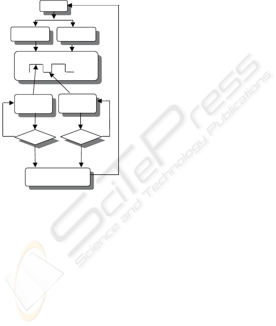
7 PROPOSED BATCH CONTROL
ALGORITHM
We have experienced several industrial process for
which the production is in two phase : a phase of
production , by the working of a material in input ,
and a phase of wait for the other material to come. In
this case we propose to apply the SPC for the
‘process variables’ during the phase of the effective
production ( say ‘batch on’ ) and to take advantage
of the waiting phase ( say ‘batch off’) for the
identification of the automation system and applying
then the SPC to the ‘control variables’. That schema
ICINCO 2009 - 6th International Conference on Informatics in Control, Automation and Robotics
374

overcome the problem of detecting if the nature of a
fault is in the process or in the automation systems,
giving a separation of the two analysis at the origin.
APC
SPC Process
Monitoring
D
etec
t
Diagnostic & Improvement
HDS Process
On Line Monitoring
HDS Control
SPC Control
Monitorin
g
D
etec
t
Y
Y
N
N
Batch on
Batch off
Figure 7: Algorithm of implementation.
When a signal of the control charts is detected
we can say if it is due to the process or to a change
of the transfer function of one of the automation
systems in the manufacturing process. The phase of
diagnostic and improvement is able then to correct
the process variable signalling ( for ex. adjusting a
temperature) or operate directly on the APC that is
controlling the automation system changed to
compensate for the change, taking advantage of the
identification made of the transfer function.
8 CONCLUSIONS
In this paper a method for monitoring on line the
behaviour of an automation system is presented. The
method has the advantage of using the identification
of the transfer function of the system , so it can be
used on the APC to compensate the changes, and
with the advantage for the SPC to provide a direct
separation of the possible causes of fault.
Results of simulations are given and finally an
implementation schema of the method in a real
process is proposed . For further researches we are
applying the algorithm proposed in a rolling-mill
plant for the production of railways, that has a
production cycle on-off like the one described in the
paper.
REFERENCES
Mason, R.L., Young, J.C., 2002. Multivariate Statistical
Process Control with Industrial Application. ASA-
SIAM.
Tsung, F., Apley, D.W., 2002. The dynamic T2 chart for
monitoring feedback-controlled processes. IIE
Transactions (2002) 34,1043-1053 IIE.
Kourti, T., MacGregor, J.F., 1994. Process analysis,
monitoring and diagnosis,using multivariate projection
methods. Chemometrics and Intelligent Laboratory
Systems 28 (1995) 3-21. ELSEVIER.
Tsung, F., 1999. Improving automatic-controlled process
quality using adaptative principal component
monitoring. Qual.Rielab.Engng.Int. 15:135-142(1999)
John Wiley & Sons;Ltd.
Ljung, L., 1987. System Identification: Theory for the
user. Prentice-Hall.
DETECTION OF A FAULT BY SPC AND IDENTIFICATION - A Method for Detecting Faults of a Process Controlled
by SPC
375