A PRACTICAL STEREO SYSTEM BASED ON REGULARIZATION

AND TEXTURE PROJECTION

Federico Tombari

1,2

and Kurt Konolige

Willow Garage Inc., Menlo Park, CA, U.S.A.

DEIS - ARCES, University of Bologna, Italy

Keywords:

Stereo vision, Spacetime stereo, Robot vision.

Abstract:

In this paper we investigate the suitability of stereo vision for robot manipulation tasks, which require high-

ﬁdelity real-time 3D information in the presence of motion. We compare spatial regularization methods for

stereo and spacetime stereo, the latter relying on integration of information over time as well as space. In both

cases we augment the scene with textured projection, to alleviate the well-known problem of noise in low-

textured areas. We also propose a new spatial regularization method, local smoothing, that is more efﬁcient

than current methods, and produces almost equivalent results. We show that in scenes with moving objects

spatial regularization methods are more accurate than spacetime stereo, while remaining computationally sim-

pler. Finally, we propose an extension of regularization-based algorithms to the temporal domain, so to further

improve the performance of regularization methods within dynamic scenes.

1 INTRODUCTION

As part of the Personal Robot project at Willow

Garage, we are interested in building a mobile robot

with manipulators for ordinary household tasks such

as setting or clearing a table. An important sensing

technology for object recognition and manipulation is

short-range (30cm – 200cm) 3D perception. Criteria

for this device include:

• Good spatial and depth resolution (1/10 degree, 1

mm).

• High speed (>10 Hz).

• Ability to deal with moving objects.

• Robust to ambient lighting conditions.

• Small size, cost, and power.

Current technologies fail on at least one of these cri-

teria. Flash ladars (Anderson et al., 2005) lack depth

and, in some cases, spatial resolution, and have non-

gaussian error characteristics that are difﬁcult to deal

with. Line stripe systems (Curless and Levoy, 1995)

have the requisite resolution but cannot achieve 10

Hz operation, nor deal with moving objects. Struc-

tured light systems (Salvi et al., 2004) are achieving

reasonable frame rates and can sometimes incorporate

motion, but still rely on expensive and high-powered

projection systems, while being sensitive to ambient

illumination and object reﬂectance. Standard block-

matching stereo, in which small areas are matched be-

tween left and right images (Konolige, 1997), fails on

objects with low visual texture.

An interesting and early technology is the use

of stereo with unstructured light (Nishihara, 1984).

Unlike structured light systems with single cameras,

stereo does not depend on the relative geometry of

the light pattern – the pattern just lends texture to the

scene. Hence the pattern and projector can be simpli-

ﬁed, and standard stereo calibration techniques can be

used to obtain accurate 3D measurements.

Even with projected texture, block-matching

stereo still forces a tradeoff between the size of the

match block (larger sizes have lower noise) and the

precision of the stereo around depth changes (larger

sizes “smear” depth boundaries). One possibility is

to use smaller matching blocks, but reduce noise by

using many frames with different projection patterns,

thereby adding information at each pixel. This tech-

nique is known as Spacetime Stereo (STS) (Davis

et al., 2005),(Zhang et al., 2003). It produces out-

standing results on static scenes and under controlled

illumination conditions, but movingobjects create ob-

vious difﬁculties (see Figure 1, bottom-left). While

there have been a few attempts to deal with mo-

tion within a STS framework (Zhang et al., 2003),

(Williams et al., 2005), the results are either compu-

Tombari F. and Konolige K.

A PRACTICAL STEREO SYSTEM BASED ON REGULARIZATION AND TEXTURE PROJECTION.

DOI: 10.5220/0002167800050012

In Proceedings of the 6th International Conference on Informatics in Control, Automation and Robotics (ICINCO 2009), page

ISBN: 978-989-674-000-9

Figure 1: The top ﬁgure shows the disparity surface for

a static scene; disparities were computed by integrating

over 30 frames with varying projected texture using block-

matching (3x3x30 block). The bottom-left ﬁgure is the

same scene with motion of the center objects, integrated

over 3 frames (5x5x3 block). The bottom-right ﬁgure is

our local smoothing method for a single frame (5x5 block).

tationally expensive or perform poorly, especially for

fast motions and depth boundaries.

In this paper, we apply regularization methods to

attack the problem of motion in spacetime stereo.

One contribution we propose is to enforce not only

spatial, but also temporal smoothness constraints that

beneﬁt from the texture-augmented appearance of the

scene. Furthermore, we propose a new regularization

method, local smoothing, that yields an interesting

efﬁciency-accuracy trade-off. Finally, this paper also

aims at comparing STS with regularization methods,

since a careful reading of the spacetime stereo liter-

ature (Davis et al., 2005; Zhang et al., 2003) shows

that this has not been addressed before. Experimen-

tally we found that, using a projected texture, regu-

larization methods applied on single frames perform

better than STS on dynamic scenes (see Figure 1) and

produces interesting results also on static scenes.

In the next section we review several standard reg-

ularization methods, and introduce our novel method,

local smoothness, which is more efﬁcient and almost

as effective. We then show how regularization can be

applied across time as well as space, to help alleviate

the problem of object motion in STS. In the experi-

mental section, the considered methods are compared

on static scenes and in the presence of moving objects.

2 SMOOTHNESS CONSTRAINTS

IN STEREO MATCHING

Stereo matching is difﬁcult in areas with low tex-

ture and at depth boundaries. Regularization meth-

ods add a smoothness constraint to model the reg-

ularity of surfaces in the real world. The general

idea is to penalize those candidates lying at a differ-

ent depth from their neighbors. A standard method

is to construct a disparity map giving the probability

of each disparity at each pixel, and compute a global

energy function for the disparity map as a multi-class

Pairwise Markov Random Field. The energy is then

minimized using approximate methods such as Belief

Propagation (BP) (Klaus et al., 2006), (Yang, 2006)

or Graph Cuts (GC) (Kolmogorov and Zabih, 2001).

Even though efﬁcient BP-based algorithms have been

proposed (Yang et al., 2006), (Felzenszwalb and Hut-

tenlocher, 2004), overall the computational load re-

quired by global approaches does not allow real-time

implementation on standard PCs.

Rather than solving the full optimization prob-

lem over the disparity map, scanline methods en-

force smoothness along a line of pixels. Initial ap-

proaches based on Dynamic Programming (DP) and

Scanline Optimization (SO) (Scharstein and Szeliski,

2002) use only horizontal scanlines, but suffer from

streaking effects. More sophisticated approaches

apply SO over multiple, variably-oriented scanlines

(Hirschmuller, 2005) or use multiple horizontal and

vertical passes (Kim et al., 2005), (M. Bleyer, 2008),

(Gong and Yang, 2005). These methods tend to be

faster than global regularization, though the use of

several DP or SO passes tends to increase the com-

putational load of the algorithms.

Another limit to the applicability of these ap-

proaches within a mobile robotic platform is their

fairly high memory requirements. This section we re-

view scanline methods and proposes a new method

called local smoothness.

2.1 Global Scanline Methods

Let I

, I

be a rectiﬁed stereo image pair sized M · N

and W(p) a vector of points belonging to a squared

window centered on p. The standard block-matching

stereo algorithm computes a local cost C(p, d) for

each point p ∈ I

and each possible correspondence

at disparity d ∈ D on I

C(p, d) =

∑

q∈W(p)

e(I

(q), I

(δ(q, d))). (1)

where δ(q, d) is the function that offsets q in I

ac-

cording to the disparity d, and e is a (dis)similarity

function. A typical dissimilarity function is the L

distance:

e(I

(q), I

(δ(q, d))) = |I

(q) − I

(δ(q, d))|. (2)

In this case, the best disparity for point p is selected

as:

∗

= argmin

{C(p, d)}. (3)

ICINCO 2009 - 6th International Conference on Informatics in Control, Automation and Robotics

In the usual SO or DP-based framework, the global

energy functional being minimized along a scanline S

is:

E (d(·)) =

∑

p∈S

C(p, d(p)) +

∑

p∈S

∑

q∈N (p)

ρ(d(p), d(q))

(4)

where d(·) denotes now a function that picks out a

disparity for its pixel argument, and q ∈ N (p) are the

neighbors of p according to a pre-deﬁned criterion.

Thus to minimize (4) one has to minimize two differ-

ent terms, the ﬁrst acting as a local evidence and the

other enforcing smooth disparity variations along the

scanline, resulting in a non-convexoptimization prob-

lem. The smoothness term ρ is usually derived from

the Potts model (Potts, 1995):

ρ(d(p), d(q)) =



0 d(p) = d(q)

π d(p) 6= d(q)

(5)

π being a penalty term inversely proportional to the

temperature of the system. Usually for stereo a Mod-

iﬁed Potts model is deployed, which is able to han-

dle slanted surfaces by means of an additional penalty

term π

<< π:

ρ(d(p), d(q)) =







0 d(p) = d(q)

|d(p) − d(q)| = 1

π elsewhere

(6)

Thanks to (6), smooth variations of the disparity

surface are permitted at the cost of the small penalty

. Usually in SO and DP-based approaches the set

of neighbours for a point p includes only the previ-

ous point along the scanline, p

−1

. From an algorith-

mic perspective, an aggregated cost A(p, d) has to be

computed for each p ∈ S, d ∈ D:

A(p, d) = C(p, d) + min

′

{A(p

−1

, d

′

) + ρ(d,d

′

)} (7)

Because of the nature of (7) the full cost for each

disparity value at the previous point p

−1

must be

stored in memory. If a single scanline is used, this

typically requires O(M · D) memory, while if mul-

tiple passes along non-collinear scanlines are con-

cerned, this usually requires O(M · N · D) memory

(Hirschmuller, 2005).

2.2 Local Smoothness

Keeping the full correlation surface over M · N · D is

expensive; we seek a more local algorithm that ag-

gregates costs incrementally. In a recent paper (Zhao

and Katupitiya, 2006), a penalty term is added in a lo-

cal fashion to improve post-processing of the dispar-

ity image based on left-right consistency check. Here,

we apply a similar penalty during the construction of

the disparity map and generalize its use for multiple

scanlines. Given a scanline S, we can modify (7) as

follows:

(p, d) = C(p, d) + ρ(d,

d) (8)

where

d = argmin

{C(p

−1

, d)} (9)

is the best disparity computed for the previous point

along the scanline. Hence, each local cost is penalized

if the previously computed correspondence along the

scanline corresponds to a different disparity value. In

this approach, there is no need to keep track of an ag-

gregated cost array, since the aggregated cost for the

current point only depends on the previously com-

puted disparity. In practice the computation of (8)

for the current disparity surface might be performed

simply by subtracting π from C(p,

d) and π− π

from

C(p,

d − 1), C(p,

d + 1).

Enforcing smoothness in just one direction helps

handle low-textured surfaces, but tends to be inaccu-

rate along depth borders, especially in the presence of

negative disparity jumps. Using two scans, e.g. hori-

zontally from left to right and from right to left, helps

to reduce this effect, but suffers from the well-known

streaking effect (Scharstein and Szeliski, 2002). In or-

der to enforce inter-scanline consistency, we run local

smoothness over 4 scans, 2 vertical and 2 horizontal

(see Figure 8). In this case, which we will refer to as

Spatial Local Smoothness (LS

), the aggregated cost

(8) is modiﬁed as follows:

(d) = C(p, d) +

∑

q∈N (p)

ρ(d, d(q)). (10)

Here N refers to the 4 disparities previously com-

puted on p. The computation of d

∗

beneﬁts from

propagated smoothness constraints from 4 different

directions, which reduces noise in low-textured sur-

faces, and also reduces streaking and smearing effects

typical of scanline-based methods.

It is worth pointing out that the LS

approach can

be implemented very efﬁciently by means of a two-

stage algorithm. In particular, during the ﬁrst stage

of the algorithm, the forward-horizontal and forward-

vertical passes are computed, and the result

is stored into two M · N arrays. Then, during the

second pass, the backward-horizontal and backward-

vertical passes are processed, and within the same

step the ﬁnal aggregated cost (10) is also computed.

Then the best disparity is determined as in (9).

Overall,

computational cost is between 3 and 4 times that

of the standard local stereo algorithm. Memory re-

quirements are also small – O(2× M × N).

A PRACTICAL STEREO SYSTEM BASED ON REGULARIZATION AND TEXTURE PROJECTION

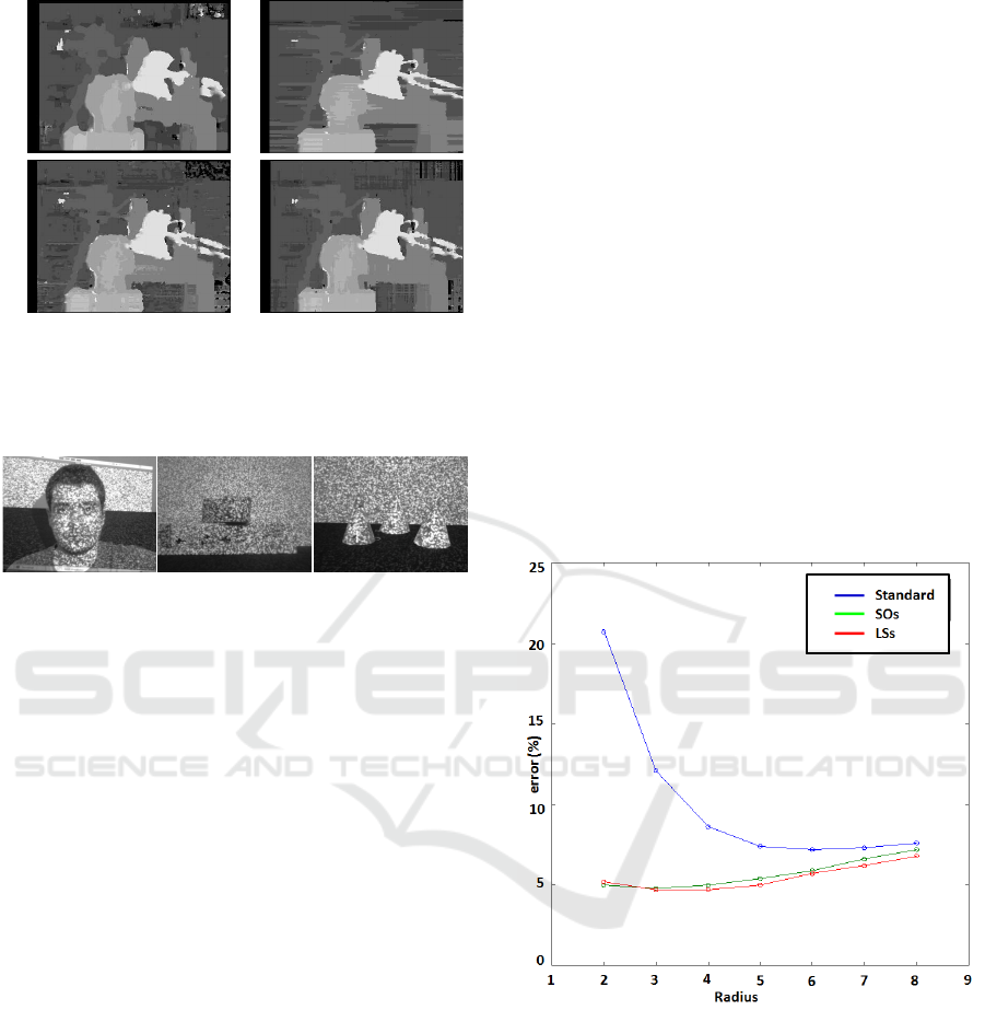
Figure 2: Qualitative comparison of different algorithms

based on the smoothness constraint: a)standard b)SO-based

c)local smoothness (2 horizontal scanlines) d)local smooth-

ness (4 scanlines).

Figure 3: Dataset used for experiments: from left to right,

Face, Cubes, Cones sequences.

2.3 Experimental Evaluation

In this section we brieﬂy present some experimen-

tal results showing the capabilities of the previously

introduced regularization methods on stereo data by

comparing them to a standard block-correlation stereo

algorithm. In particular, in addition to the LS

algo-

rithm, we consider a particularly efﬁcient approach

based only on one forward and one backward hori-

zontal SO pass (M. Bleyer, 2008). This algorithm ac-

counts for low memory requirements and fast perfor-

mance, though it tends to suffer the streaking effect.

We will refer to this algorithm as SO

Fig. 2 shows some qualitative results on the

Tsukuba dataset (Scharstein and Szeliski, 2002). The

standard local algorithm is in (a), SO

(b) and the LS

algorithm in (d). Also, the ﬁgure shows the disparity

map obtained by the use of the Local Smoothness cri-

terion over only 2 horizontal scanlines in (c). It can

be noticed that, compared to the standard approach,

regularization methods allow for improved accuracy

along depth borders. Furthermore, while methods

based only on horizontal scanlines (b, c) present typ-

ical horizontal streaking effects, these are less notice-

able in the LS

algorithm (d). In our implementation,

using standard incremental techniques but no SIMD

or multi-thread optimization, time requirements on a

standard PC for the standard, SO

and LS

algorithms

are 18, 62 and 65 ms, respectively.

In addition, we show some results concerning im-

ages where a pattern is projected on the scene. As for

the pattern, we use a randomly-generated grayscale

chessboard, which is projected using a standard video

projector. Fig. 3 shows 3 frames taken from 3 stereo

sequences used here and in Section 3.4 for our ex-

periments. Sequence Face is a static sequence, while

Cubes and Cones are dynamic scenes where the ob-

jects present in the scene rapidly shift towards one

side of the table. All frames of all sequences are

640× 480 in resolution.

Figure 4 shows experimental results for the stan-

dard algorithm as well as SO

and LS

over different

window sizes. Similarly to what done in (Davis et al.,

2005), ground truth for this data is the disparity map

obtained by the spacetime stereo technique (see next

Section) over all frames of the sequence using a 5× 5

window patch. A point in the disparity map is con-

sidered erroneous if the absolute difference between

it and the groundtruth is higher than one.

Figure 4: Quantitative comparison between different spatial

approaches: standard algorithm, SO

, LS

From the ﬁgure it is clear that, even on this real

dataset, regularization methods allow for improved

results compared to standard methods since the curve

concerningthe standard algorithm is always abovethe

other two. It is worth pointing out that both SO

and

achievetheir minimum with a smaller spatial win-

dow compared to the standard algorithm, allowing for

reduced smearing effect along depth borders. Con-

versely, the use of regularization methods with big

windows increase the error rate which tends to con-

verge to the one yielded by the standard method. It is

ICINCO 2009 - 6th International Conference on Informatics in Control, Automation and Robotics

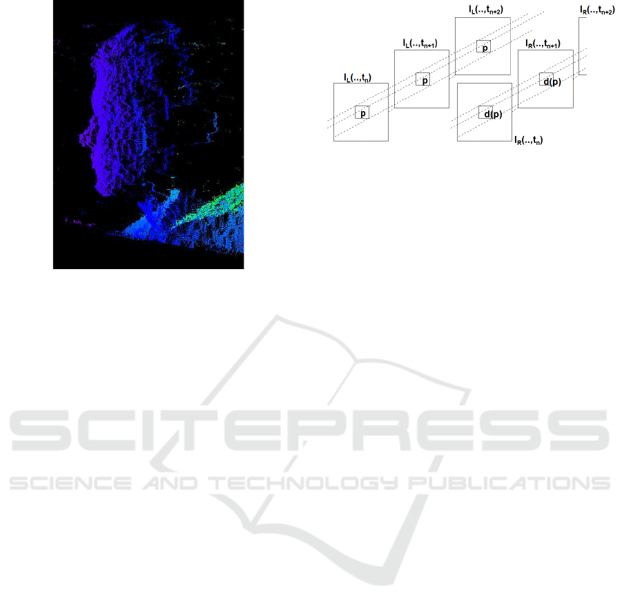
Figure 5: Point cloud showing the 3D proﬁle of the face in

Fig. 3 (left), computed using a single frame and LS

algo-

rithm.

also worth pointing out that overall the best result is

yielded by the proposed LS

algorithm. Finally, Fig-

ure 5 shows the 3D point cloud of the face proﬁle

obtained by using the LS

algorithm over one frame

on the Face dataset. From the Figure it can be noted

that despite being fast and memory-efﬁcient, this al-

gorithm is able to obtain good accuracy in the recon-

structed point cloud.

3 SPACETIME STEREO

Block-correlation stereo uses a spatial window to

smooth out noise in stereo matching. A natural ex-

tension is to extend the window over time, that is, to

use a spatio-temporal window to aggregate informa-

tion at a pixel (Zhang et al., 2003), (Davis et al., 2005)

(Figure 6). The intensity at position I(p, t) is now de-

pendent on time, and the block-matching sum over a

set of frames F and a spatial windowW can be written

C(p, d) =

∑

t∈F

∑

q∈W(p)

e(I

(q,t), I

(δ(q),t)). (11)

Minimizing C over d yields an estimated disparity at

the pixel p. Note that we obtain added information

only if the scene illumination changes within F.

As pointed out in (Zhang et al., 2003), block

matching in Equation (11) assumes that the dispar-

ity d is constant over both the local neighborhood W

and the frames F. Assuming for the moment that the

scene is static, by using a large temporal window F

Figure 6: Spacetime window for block matching. Spatial

patches centered on p are matched against corresponding

patches centered on d(p), and the results summed over all

frames.

we can reduce the size of the windowW while still re-

ducing matching noise. This strategy has the further

salutary effect of minimizing the smearing of object

boundaries. Figure 1 (top) shows a typical result for

spacetime block matching of a static scene with small

spatial windows.

3.1 Moving Objects

In a scene with moving objects, the assumption of

constant d over F is violated. A simple scheme to

deal with motion is to trade off between spatial and

temporal window size (Davis et al., 2005). In this

method, a temporal window of the last k frames is

kept, and when a new frame is added, the oldest frame

is popped off the window, and C(p, d) is calculated

over the last k frames. We will refer to this approach

as sliding windows (STS-SW). The problem is that

any large image motion between frames will com-

pletely erase the effects of temporal integration, es-

pecially at object boundaries (see Figure 1, bottom-

left). It is also suboptimal, since some areas of the

image may be static, and would beneﬁt from longer

temporal integration.

A more complex method is to assume locally lin-

ear changes in disparity over time, that is, d(p,t) is a

linear function of time (Zhang et al., 2003):

d(p,t) ≈ d(p,t

) + α(p)(t − t

). (12)

For smoothly-varying temporal motion at a pixel, the

linear assumption works well. Unfortunately, search-

ing over the space of parameters α(p) makes min-

imizing the block-match sum (11) computationally

difﬁcult. Also, the linear assumption is violated at

the boundaries of moving objects, where there are

abrupt changes in disparity from one frame to the next

(see Figure 7). These temporal boundaries present the

same kind of challenges as spatial disparity bound-

aries in single-frame stereo.

A PRACTICAL STEREO SYSTEM BASED ON REGULARIZATION AND TEXTURE PROJECTION

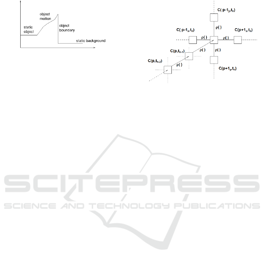
Figure 7: Disparity at a single pixel during object mo-

tion. Initially disparity is constant (no motion); then varies

smoothly as the object moves past the pixel. At the object

boundary there is an abrupt change of disparity.

A more sophisticated strategy would be to detect

the temporal boundaries and apply temporal smooth-

ness only up to that point. In this way, static im-

age areas enjoy long temporal integration, while those

with motion use primarily spatial information. Hence,

we propose a novel method with the aim of ef-

ﬁciently dealing with dynamic scenes and rapidly-

varying temporal boundaries. In particular, the main

idea is to avoid using the spacetime stereo formula-

tion as in (11) which blindly averages all points of the

scene over time, instead enforcing a temporal smooth-

ness constraint similarly to what is done spatially.

In particular, this can be done either modelling the

spatio-temporal structure with a MRF and solving us-

ing an SO or DP-based approach, or enforcing a local

smoothness constraint as described in Section 2.

3.2 Temporal Regularization using SO

The idea of looking for temporal discontinuities was

ﬁrst discussed in (Williams et al., 2005), which pro-

posed an MRF framework that extends over three

frames. The problem with this approach is that the

cost in storage and computation is prohibitive, even

for just 3 frames. Here we propose a much more efﬁ-

cient method that consists in deﬁning a scanline over

time, analogous to the SO method over space. Given

a cost array for each point and time instant C(p, d,t)

being computed by means of any spatial method (lo-

cal, global, DP-based, ··· ), a SO-based approach is

used for propagating forward a smoothness constraint

over time:

(p, d,t) = C(p, d,t) + min

′

(p, d

′

,t − 1) + ρ(d,d

′

)}

(13)

Instead of backtracking the minimum cost path as in

the typical DP algorithm, here it is more convenient

to compute the best disparity over space and time as

follows:

∗

(p,t) = argmin

(p, d,t)} (14)

so that for each new frame its respective disparity im-

age can be readily computed. As shown in Figure

Figure 8: Local smoothing applied in the temporal domain.

Disparity values inﬂuence the center pixel at time t

from

vertical and horizontal directions, and also from previous

frames t

, i < n.

8, accumulated costs from previous frames t

i<n

are

propagated forward to inﬂuence the correlation sur-

face at time t

. Here we propose to use as spatial algo-

rithm the SO-based approach deploying two horizon-

tal scanlines as discussed in Section 2. This algorithm

is referred to as SO

s,t

3.3 Temporal Regularization using

Local Smoothness

In a manner similar to applying SO across frames, we

can instead use local smoothness. The key idea is to

modify the correlation surface at position p and time t

according to the best disparity found at the same point

p at the previous instant t − 1. This does not require

storing and propagating a cost array, only the corre-

spondences found at the previous time instant.

The local temporal smoothness criterion is orthog-

onal to the strategy adopted for solving stereo over the

spatial domain, hence any local or global stereo tech-

niques can be used together with it. Here we propose

to use local spatial smoothness described in Section

2. The cost function at pixel p and time t becomes:

s,t

(p, d,t) = C(p, d,t) +

∑

q∈N

ρ(d, d(q,t)) + ρ(d, d(p,t − 1)), (15)

That is, the penalty terms added to the local cost are

those coming from the 4 independent scanline-based

processes at time t plus an additional one that depends

on the best disparity computed at position p at the

previous time instant (see Figure 8). This algorithm

will be referred to as LS

s,t

It is possible to propagate information both for-

wards and backwards in time, but there are several

reasons for only going forwards. First, it keeps the

ICINCO 2009 - 6th International Conference on Informatics in Control, Automation and Robotics

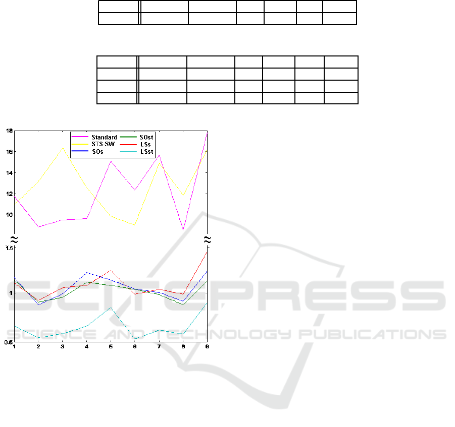
Table 1: Percentage of errors, Cubes stereo sequence.

Radius STS-SW Standard SO

s,t

LSs, t

2 12.8 12.1 1.1 1.0 1.1 0.7

Table 2: Percentage of errors, Cones stereo sequence.

Radius STS-SW Standard SO

s,t

LSs, t

1 46.9 49.9 5.3 5.2 14.8 12.2

3 35.4 15.9 4.2 4.1 8.2 6.9

5 31.9 9.6 4.6 4.5 7.0 6.1

Figure 9: Comparison of error percentages between differ-

ent approaches for the Cubes sequence at each frame of the

sequence. [The graph uses two different scales for better

visualization].

data current – previous frames may not be useful for a

realtime system. Second, the amount of computation

and storage is minimal for forward propagation. Only

the previous image local costs have to be maintained,

which is O(M · N). In contrast, to do both forwards

and backwards smoothing we would need to save lo-

cal costs over k frames (O(k · M · N)), and worse, re-

compute everything for the previous k frames, where

k is the size of the temporal window for accumulation.

3.4 Experiments

This section presents experimental results over two

stereo sequences with moving objects and a projected

pattern, referred to as Cubes and Cones (see Fig. 3).

To obtain ground truth for the stereo data, each differ-

ent position of the objects is captured over 30 frames

with a 3× 3 spatial window, and stereo depths are av-

eraged over time by means of spacetime stereo. Then,

a sequence is built up by using only one frame for

each different position of the objects.

As a comparison, we compute spacetime stereo

using the sliding window approach (STS-SW). This

approach is compared with regularization techniques

based only on spatial smoothness (i.e. SO

, LS

) as

well as with those enforcing temporal regularization

(i.e. SO

s,t

, LS

s,t

Figure 9 shows the error rates of each algorithm

for each frame of the Cubes dataset, with a ﬁxed spa-

tial window of radius 2. Table 1 reports the average

error over the whole sequence. In addition, Figure 1

shows the ground truth for one frame of the sequence

as well as the results obtained by STS− SW and LS

s,t

As can be seen, due to the rapid shift of the objects in

the scene, the approach based on spacetime stereo is

unable to improve the results compared to the stan-

dard algorithm. Instead, approaches based on spa-

tial regularization yield very low error rates, close to

those obtained by the use of spacetime stereo over the

same scene but with no moving objects. Furthermore,

Figure 9 shows that the error variance of the methods

enforcing the smoothness constraint is notably lower

than that reported by the standard and STS-SW algo-

rithms. It is worth pointing out that the use of the

proposed LS regularization technique both in space

and time yields the best results over all the considered

frames.

As in the previous experiment, Table 2 shows the

mean error percentages over the Cones dataset with

different spatial windows (i.e., radius 1, 3, and 5).

Also in this case, regularization approaches achieve

notably lower error rates compared to standard and

spacetime approaches. From both experiments it is

possible to observe that the introduction of temporal

smoothness always helps improving the performance

of the considered regularization methods.

A PRACTICAL STEREO SYSTEM BASED ON REGULARIZATION AND TEXTURE PROJECTION

4 CONCLUSIONS AND FUTURE

WORK

In this paper we investigated the capabilities of a

3D sensor comprised of a stereo camera and a tex-

ture projector. With off-the-shelf hardware and un-

der real illumination conditions, we have shown that

in the presence of moving objects single-frame stereo

with regularization produces much better results than

STS. Moreover, the proposed regularization approach

based on local smoothness, though not based on a

global optimization, shows good performance and

reduced computational requirements. Finally, we

have found that the proposed introduction of tempo-

ral smoothness helps improving the performance of

the considered regularization methods.

We are currently actively developing a small, low-

power stereo device with texture projection. There

are two tasks that need to be accomplished. First,

we are trying to optimize the local smoothness con-

straint to be real time on standard hardware, that is,

to run at about 30 Hz on 640x480 images. Second,

we are designing a small, ﬁxed pattern projector that

will replace the video projector. The challenge here

is to project enough light while staying eye-safe and

having a compact form factor. Using the methods de-

veloped in this paper, we believe we can make a truly

competent realtime 3D device for near-ﬁeld applica-

tions.

The code concerning the regularization methods

and the STS algorithms used in this paper is open

source and available online

REFERENCES

Anderson, D., Herman, H., and Kelly, A. (2005). Experi-

mental characterization of commercial ﬂash ladar de-

vices. In Int. Conf. of Sensing and Technology.

Curless, B. and Levoy, M. (1995). Better optical triangula-

tion through spacetime analysis. In ICCV.

Davis, J., Nehab, D., Ramamoorthi, R., and Rusinkiewicz,

S. (2005). Spacetime stereo: a unifying framework

dor depth from triangulation. IEEE Transactions on

Pattern Analysis and Machine Intelligence, 27(2).

Felzenszwalb, P. and Huttenlocher, D. (2004). Efﬁcient be-

lief propagation for early vision. In Proc. CVPR, vol-

ume 1, pages 261–268.

Gong, M. and Yang, Y. (2005). Near real-time reliable

stereo matching using programmable graphics hard-

ware. In Proc. CVPR, volume 1, pages 924–931.

Hirschmuller, H. (2005). Accurate and efﬁcient stereo pro-

cessing by semi-global matching and mutual informa-

tion. In Proc. CVPR, volume 2, pages 807–814.

prdev.willowgarage.com/trac/personalrobots/browser/pkg/trunk/vision/

Kim, J., Lee, K., Choi, B., and Lee, S. (2005). A dense

stereo matching using two-pass dynamic program-

ming with generalized ground control points. In Proc.

CVPR, pages 1075–1082.

Klaus, A., Sormann, M., and Karner, K. (2006). Segment-

based stereo matching using belief propagation and a

self-adapting dissimilarity measure. In Proc. ICPR,

volume 3, pages 15–18.

Kolmogorov, V. and Zabih, R. (2001). Computing visual

correspondence with occlusions via graph cuts. In

Proc. ICCV, volume 2, pages 508–515.

Konolige, K. (1997). Small vision systems: hardware and

implementation. In Eighth International Symposium

on Robotics Research, pages 111–116.

M. Bleyer, M, G. (2008). Simple but effective tree struc-

tures for dynamic programming-based stereo match-

ing. In Proc. Int. Conf. on Computer Vision Theory

and Applications (VISAPP), volume 2.

Nishihara, H. K. (1984). Prism: A practical real-time imag-

ing stereo matcher. Technical report, Cambridge, MA,

USA.

Potts, R. (1995). Some generalized order-disorder transi-

tions. In Proc. Cambridge Philosophical Society, vol-

ume 48, pages 106–109.

Salvi, J., Pages, J., and Batlle, J. (2004). Pattern dociﬁ-

cation strategies in structured light systems. Pattern

Recognition, 37(4).

Scharstein, D. and Szeliski, R. (2002). A taxonomy and

evaluation of dense two-frame stereo correspondence

algorithms. Int. J. Computer Vision, 47(1/2/3):7–42.

Williams, O., Isard, M., and MacCormick, J. (2005). Es-

timating disparity and occlusions in stereo video se-

quences. In Proc. CVPR.

Yang, Q., Wang, L., Yang, R., Wang, S., Liao, M., and Nis-

ter, D. (2006). Real-time global stereo matching using

hierarchical belief propagation. In Proc. British Ma-

chine Vision Conference.

Yang, Q. e. a. (2006). Stereo matching with color-weighted

correlation, hierachical belief propagation and occlu-

sion handling. In Proc. CVPR, volume 2, pages 2347

– 2354.

Zhang, L., Curless, B., and Seitz, S. (2003). Spacetime

stereo: shape recovery for dynamic scenes. In Proc.

CVPR.

Zhao, J. and Katupitiya, J. (2006). A fast stereo vision al-

gorithm with improved performance at object borders.

In Proc. Int. Conf. on Intelligent Robots and Systems

(IROS), pages 5209–5214.

ICINCO 2009 - 6th International Conference on Informatics in Control, Automation and Robotics