A NEW LIKELIHOOD FUNCTION FOR STEREO MATCHING
How to Achieve Invariance to Unknown Texture, Gains and Offsets?
Sanja Damjanovi´c, Ferdinand van der Heijden and Luuk J. Spreeuwers
Chair of Systems and Signals, Faculty of EEMCS, University of Twente, Drienerlolaan 5, Enschede, The Netherlands
Keywords:
Likelihood, NCC, Probabilistic framework, HMM, Stereo reconstruction.
Abstract:
We introduce a new likelihood function for window-based stereo matching. This likelihood can cope with
unknown textures, uncertain gain factors, uncertain offsets, and correlated noise. The method can be fine-
tuned to the uncertainty ranges of the gains and offsets, rather than a full, blunt normalization as in NCC
(normalized cross correlation). The likelihood is based on a sound probabilistic model. As such it can be
directly used within a probabilistic framework. We demonstrate this by embedding the likelihood in a HMM
(hidden Markov model) formulation of the 3D reconstruction problem, and applying this to a test scene. We
compare the reconstruction results with the results when the similarity measure is the NCC, and we show that
our likelihood fits better within the probabilistic frame for stereo matching than NCC.
1 INTRODUCTION
Stereo correspondence is the process of finding pairs
of matching points in two images that are generated
by the same physical 3D surface in space, (Faugeras,
1993). The classical approach is to consider image
windows around two candidate points, and to eval-
uate a similarity measure (or dissimilarity measure)
between the pixels inside these windows. Such an ap-
proach is based on the constant brightness assumption
(CBA) stating that, apart from noise, the image data in
two matching windows are equal. If the noise is white
and additive, then the SSD measure (sum of squared
differences), or the SAD (sum of absolute differences)
is appropriate. Often, the gains and offsets with which
the two images are acquired are not equal, and are not
precisely known. Therefore, another popular similar-
ity measure is the NCC (normalized cross correlation)
which neutralizes these offsets and gains. An alterna-
tive is the mutual information, (Egnal, 2000), which
is even invariant to a bijective mapping between the
grey levels of the left and right images.
In a probabilistic approach to stereo correspon-
dence, the similarity measures become likelihood
functions being the probability density of the ob-
served data given the ground truth. For the applica-
tion of stereo correspondence (and related to that mo-
tion estimation) several models have been proposed
for the development of the likelihood function, but
none of them consider the situation of uncertain gains
and offsets. In this paper, we introduce a new likeli-
hood function in which the unknown texture, and the
uncertainties of gains and offsets are explicitly mod-
elled.
The solution of stereo correspondence is often
represented by a disparity map. The disparity is
the difference in position between two correspond-
ing points. In the classical approach, the disparity
map is estimated point by point on an individual base.
Better results are obtained by raising additional con-
straints in the solution space. For instance, neigh-
bouring disparities should be smooth (except on the
edge of an occlusion), unique, and properly ordered.
Context-dependent approaches, such as dynamic pro-
gramming (Cox et al., 1996) and graph-cut algorithms
(Roy and Cox, 1998), embed these contextual con-
straints by raising an optimization criterion that con-
cerns a group of disparities at once, rather than in-
dividual disparities. For that purpose, an optimization
criterion is defined that expresses both the compliance
of a solution with the constraints, and the degree of
agreement with the observed image data.
The Bayesian approach has proved to be a sound
base to formulate the optimization problem on (Cox
et al., 1996; Belhumeur, 1996). Here, the optimiza-
tion criterion is expressed in terms of probability den-
sities. A crucial role is the likelihood function, i.e. the
conditional probability density of the data given the
disparities. Suppose that a given point has a disparity
x, and that for that particular point and disparity the
603
van der Heijden F., J. Spreeuwers L. and Damjanovic S. (2009).
A NEW LIKELIHOOD FUNCTION FOR STEREO MATCHING - How to Achieve Invariance to Unknown Texture, Gains and Offsets?.
In Proceedings of the Fourth International Conference on Computer Vision Theory and Applications, pages 603-608
DOI: 10.5220/0001793606030608
Copyright
c
 SciTePress

pixels in the corresponding image windows are given
by z
1
and z
2
. Then the likelihood function of that
point is by definition the pdf p(z
1
,z
2
|x).
The usual expression for this likelihood is again
based on the CBA, and assumes Gaussian, additive
white noise. Application of this model leads to the
following likelihood:
p(z
1
,z
2
|x) ∝ exp

−
1
4σ
2
n
kz
1
−z
2
k
2

(1)
Here, kz
1
−z
2
k
2
is the SSD. The likelihood function
in eq. (1) is a monotonically decreasing function of
the SSD. It is used by (Cox et al., 1996) and (Bel-
humeur, 1996) albeit that both have an additional pro-
vision for occluded pixels. However, the function is
inappropriate if the gains and offsets are uncertain.
Yet, the differences between the grey levels in two
corresponding windows is often more affected by dif-
ferences in gains and offsets than by noise. This paper
introducesnew expressions which do include these ef-
fects. The NCC and the mutual information similarity
measures are also invariant to these nuisance factors.
However, these measures are parameters derivedfrom
the pdfs. But in a true probabilistic approach we really
need the pdfs themselves, and not just parameters.
The paper is organized as follows. Section 2 in-
troduces the new likelihood function. Here, a prob-
abilistic model is formulated that explicitly describes
the existence of an unknown texture, and uncertain
gains and offsets. The final likelihood is obtained
by marginalization of these factors. Section 3 anal-
yses the expression that is found for the likelihood.
In Section 4, we present some experimental results
where the likelihood function is used within a HMM
framework. A comparison is made between the newly
derived likelihood and the NCC when used in a for-
ward/backward algorithm. Section 5 gives conclud-
ing remarks and further directions.
2 THE LIKELIHOOD OF TWO
CORRESPONDING POINTS
We consider two corresponding points with dispar-
ity x. The image data within two windows that sur-
round the two points are represented by z
1
and z
2
.
The grey levels (or colours) within the windows de-
pend on the texture and radiometric properties of the
observed surface patch, but also on the illumination
of the surface, and on the properties of the imaging
device. We model this by:
z
k
= α
k
s+ n
k
+ β
k
e k = 1,2 (2)
Here, s is the result of mapping the texture on the sur-
face to the two image planes. According to the CBA,
this mapping yields identical results in the two im-
ages. α
k
are the gain factors of the two imaging de-
vices. β
k
are the offsets. e is the all 1 vector. n
k
are
noise vectors. We assume Gaussian noise with co-
variance matrix C
n
. Furthermore, we assume that n
1
is not correlated with n
2
.
Strictly speaking, the CBA can only hold for
fronto-parallel planar surface patches. In all other
cases the local geometry of the surface around a point
of interest is mapped differently to the two image
planes. Thus, the texture on the surface will be ob-
served differently in the images. This problem be-
comes more distinct as the size of the window in-
creases. The problem can be solved by backmap-
ping the image data within the two windows to the
3D surface before applying the similarity measure,
(Spreeuwers, 2008). In the sequel, we will assume
that either such a geometric correction has taken
place, or that the windows are so small that the aper-
ture problem can be neglected.
In order to get the expression for the likelihood
function we marginalize the pdf of z
1
and z
2
with re-
spect to the unknown texture s. Next, we marginalize
the resulting expression with respect to the gains α
k
.
The offsets can be dealt with by regarding n
k
+ β
k
e
as one additive noise term. Thus, a redefinition of C
n
suffices. This will be looked upon in more detail in
Section 2.3, but for the moment we can ignore the ex-
istence of offsets.
2.1 Texture Marginalization
The likelihood function can be obtained by marginal-
ization of the texture:
p(z
1
,z
2
|x,α
1
,α
2
) =
Z
s
p(z
1
,z
2
|x,s,α
1
,α
2
)p(s|x)ds
(3)
The pdf p(s|x) represents the prior pdf of the texture s.
For simplicity, we assume a full lack of prior knowl-
edge, thus leading to a prior pdf which is constant
within the allowable range of z
1
and z
2
. This justi-
fies the following simplification:
p(z
1
,z
2
|x) = K
Z
s
p(z
1
,z
2
|x,s,α
1
,α
2
)ds (4)
K is a normalization constant that depends on the
width of p(s). Any width will do as long as p(s) cov-
ers the range of interest of z
1
and z
2
. Therefore, K is
undetermined. This is not really a limitation since K
does not depend on x, z
1
or z
2
.
With s fixed, z
1
and z
2
are two uncorrelated, nor-
mal distributed random vectors with mean s, and co-
VISAPP 2009 - International Conference on Computer Vision Theory and Applications
604

variance matrix C
n
. Therefore p(z
1
,z
2
|x,α
1
,α
2
) =
G(z
1
−α
1
s)G(z
2
−α
2
s), where G(·) is a Gaussian
distribution with zero mean and covariance matrix
C
n
. This expression can be further simplified by the
introduction of two auxiliary variables: h ≡
z
1
α
1
−s
and y ≡
z
1
α
1
−
z
2
α
2
so that h−y =
z
2
α
2
−s. The likeli-
hood function can be obtained by substitution:
p(z
1
,z
2
|x,α
1
,α
2
) = K
Z
h
G(α
1
h)G(α
2
(h−y))dh
and by rewriting this in the Gaussian form:
p(z
1
,z
2
|x,α
1
,α
2
) ∝
1
√
α
2
1
+α
2
2
exp

−
(α
2
z
1
−α
1
z
2
)
T
C
n
−1
(α
2
z
1
−α
1
z
2
)
2(α
2
1
+α
2
2
)

(5)
Note that for α
1
= α
2
= 1 and C
n
= σ
2
n
I the likelihood
simplifies to eq. (1). The resulting likelihood function
is the same as in (Cox et al., 1996; Belhumeur, 1996)
although the models on which the expression is based
differ.
2.2 Marginalization of the Gains
In order to neutralize the unknowngains we marginal-
ize over α
1
and α
2
:
p(z
1
,z
2
|x) =
Z
α
1
Z
α
2
p(z
1
,z
2
|x,α
1
,α
2
)p(α
1
)p(α
2
)dα
2
dα
1
(6)
The prior pdfs p(α
k
) should reflect the prior knowl-
edge about the gains α
k
. Usually, the gain factors
do not deviate too much from 1. For that reason, we
chose for p(α
k
) a normal distribution, centred around
1, and with standard deviations σ
α
. In order to make
the analytical integration of eq. (5) possible, we ap-
proximate the term 1/(α
2
1
+α
2
2
) by its value at α
k
= 1,
that is
1
2
. This approximation is rough, but not too
rough. For α
k
< 1, the factor 1/(α
2
1
+ α
2
2
) is under-
estimated, but for α
k
> 1 it is overestimated. Since
the integration takes place on both side of α
k
= 1, the
error is partly compensated for.
Under the assumption α
k
∼ N(1,σ
α
), the approx-
imation leads to the following result:
p(z
1
,z
2
|x) ∝
exp

−
σ
2
α
(ρ
11
ρ
22
−ρ
2
12
)+ρ
11
+ρ
22
−2ρ
12
σ
4
α
(ρ
11
ρ
22
−ρ
2
12
)+2σ
2
α
(ρ
11
+ρ
22
)+4

q
σ
4
α
(ρ
11
ρ
22
−ρ
2
12
) + 2σ
2
α
(ρ
11
+ ρ
22
) + 4
(7)
where:
ρ
kℓ
= z
T
k
C
−1
n
z
ℓ
with : k,ℓ = 1, 2 (8)
In the limiting case, as σ
α
→ 0, we have
p(z
1
,z
2
|x) ∝ exp

−
1
4
(ρ
11
+ ρ
22
−2ρ
12
)

(9)
which coincides with eq. (1). Intuitively, this is cor-
rect since the uncertainties about α
1
and α
2
is zero
then. In the other limiting case, as σ
α
→ ∞, the like-
lihood becomes:
p(z
1
,z
2
|x) ∝
1
q
ρ
11
ρ
22
−ρ
2
12
(10)
We will analyse these expressions further in Section
3.
2.3 Neutralizing the Unknown Offsets
We assume that the offsets β
k
have a normal distribu-
tion with zero mean, and standard deviation σ
β
. The
vectors β
k
e have a covariance matrix σ
2
β
ee
T
. Since
the random vectors are additive, we may absorb them
in the noise vectors n
k
. Effectively this implies that
the covariance matrix C
n
now becomes C
n
+ σ
2
β
ee
T
.
Consequently, the variable ρ
kℓ
in eq. (8) should be
redefined by ρ
kℓ
= z
T
k
(C
n
+ σ
2
β
ee
T
)
−1
z
ℓ
This can be
rewritten in:
ρ
kℓ
= z
T
k
N
∑
n=1
v
n
λ
−1
n
v
T
n
!
z
ℓ
(11)
λ
n
are the eigenvaluesof the covariance matrix. v
n
are
the corresponding eigenvectors. Suppose that Nσ
2
β
is
large relative to all other eigenvalues of C
n
(N is the
dimension of z
k
). In case of white noise, the equiva-
lent assumption is Nσ
2
β
≫σ
2
n
). Then one of the eigen-
values of C
n
+ σ
2
β
ee
T
is close to Nσ
2
β
, while all other
eigenvaluesare considerably smaller. The eigenvector
that corresponds to σ
2
β
is close to e. The contribution
of this particular eigenvalue/eigenvector to ρ
kℓ
in eq.
(11) is about:
z
T
k
ee
T
z
ℓ
Nσ
2
β
. (12)
The limit case, σ
β
→ ∞, represents the situation of
full lack of prior knowledge of the offsets. In this cir-
cumstance, the approximations above become exact.
Thus, the full contribution in eq. (12 ) becomes zero.
There is no need to embed σ
2
β
ee
T
in C
n
. The fac-
tor z
T
k
e is the projection of z
k
on e. We just need to
remove this projection from z
k
beforehand, and then
its contribution is zero anyhow. This can be obtained
by subtracting the average of the elements of the vec-
tor. Thus, if ¯z
k
is the average of the elements of the
vector z
k
, then:
ρ
kℓ
= (z
k
−¯z
k
e)
T
C
−1
n
(z
ℓ
−¯z
ℓ
e) (13)
Note that this approach to cope with unknown offsets
is equivalent to the normalization of the mean, just as
in the NCC procedure.
A NEWLIKELIHOOD FUNCTION FOR STEREO MATCHING - How to Achieve Invariance to Unknown Texture, Gains
and Offsets?
605

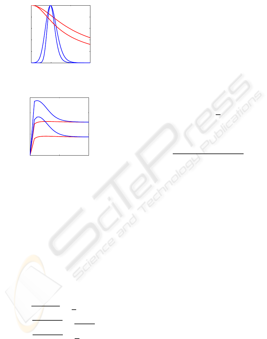
0 1 2 3
0
0.2
0.4
0.6
0.8
1
α
1
→
normalized likelihood
a)
b)
c)
d)
a) σ
α
→∞, σ
s
=1
b) σ
α
→∞, σ
s
=100
c) σ
α
=0.1, σ
s
=1
d) σ
α
=0.1, σ
s
=100
Figure 1: The likelihood function with varying α
1
. Other
parameters are: α
2
= 1, σ
n
= 1, N = 225
1 100 10000
1
10
100
N →
likelihood ratio
a)
b)
c)
d)
a) σ
α
=∞, σ
s
=10
b) σ
α
=∞, σ
s
=50
c) σ
α
=0.5, σ
s
=10
d) σ
α
=0.5, σ
s
=50
Figure 2: The likelihood ratio with varying N. Other pa-
rameters are: α
1
= 1, α
2
= 1, σ
n
= 1
3 LIKELIHOOD ANALYSIS
In this section, we examine the behaviour of the pro-
posed likelihood in different circumstances. For sim-
plicity, we consider only the white noise case, C
n
=
σ
2
n
I. First we examine the behaviour of the likelihood
function under the null hypothesis with varying α
1
.
Other parameters are kept constant. Substitution of
eq. (2) in eq. (8) yields:
ρ
kk
= (α
2
k
s
T
s+ 2α
k
s
T
n
k
+ n
T
k
n
k
)/σ
2
n
ρ
12
= (α
1
α
2
s
T
s+ α
1
s
T
n
1
+ α
2
s
T
n
2
+ n
T
1
n
2
)/σ
2
n
(14)
We regard s as a nonrandom signal. The energy σ
s
is
defined as σ
2
s
≡s
T
s/N. We examine the behaviour by
replacing the inner products in eq. (14) by their root
mean squares. That is:
s
T
n
k
∼
r
E
h
(s
T
n
k
)
2
i
=
√
Nσ
s
σ
n
n
T
k
n
k
∼
r
E
h

n
T
k
n
k

2
i
=
√
N
2
+ 2Nσ
2
n
n
T
1
n
2
∼
r
E
h

n
T
1
n
2

2
i
=
√
Nσ
2
n
(15)
Figure 1 shows the likelihood function p(z
1
,z
2
|x) for
σ
α
= ∞, conform eq. (10), and for σ
α
= 0.1, con-
form eq. (7) for varying α
1
. Of course, a substitution
by RMSs is not exact, but nevertheless, the resulting
figure gives a good impression of the behaviour. As
expected, if σ
α
is very large, the likelihood function
covers a wide range of α
1
. If σ
α
is small, then the
function is narrowly peaked around α
1
= 1.
In order to check whether the new likelihood func-
tion is able to distinguish between similar textures and
dissimilar textures, we also examined the ratio of the
likelihood function under these two different cases.
For that purpose, we also considered the alternative
model:
z
k
= α
k
s
k
+ n
k
+ β
k
e k = 1,2 (16)
In this situation, s
1
and s
2
are two different textures,
but with the same signal energy σ
s
. If we model s
1
and s
2
as realizations from two independent random
signals, then E[(s
T
1
s
2
)
2
]
1/2
= σ
2
s
√
N. Thus, if the tex-
tures are dissimilar, the RMS of the factor s
T
s in ρ
12
in eq. (14) should be replaced accordingly. The ratio
between the likelihoods in the two cases is:
Λ(z
1
,z
2
) ≡
p(z
1
,z
2
|x,similartextures)
p(z
1
,z
2
|x,dissimilartextures)
(17)
Figure 2 shows this ratio for varying N. We see that
the ratio’s with σ
α
= 0.5 are always larger than the
one with σ
α
= ∞, but for large N the ratio’s with
σ
α
= 0.5 approaches the other one and becomes con-
stant on the long run. The reason for this typical be-
haviour is that in the factor ρ
11
ρ
22
−ρ
2
12
the contribu-
tion of the signal α
1
α
2
s
T
s is cancelled out, while the
contribution of the noise, i.e. n
T
k
n
k
, is proportional to
N, and thus keeps growing as N increases.
4 EXPERIMENTS
A preliminary experiment is conducted to demon-
strate the abilities of our newly proposed likelihood.
For that purpose, two rectified stereo images were se-
lected. See Figure 3. In order to embed the likeli-
hood function within a probabilistic framework, we
treat the stereo correspondence along the epipolar line
as a state estimation problem using a HMM (Hidden
Markov Model). The reconstruction is done using the
FwBw (forward-backward) algorithm (van der Heij-
den et al., 2004). The Viterbi algorithm is also appli-
cable, but in our experiments, FwBw outperformed
Viterbi. We calculated the disparity map using the
new likelihood function as the observation probabil-
ity, and compared this map with a map obtained from
the same HMM, but with an other likelihood function
plugged in.
VISAPP 2009 - International Conference on Computer Vision Theory and Applications
606

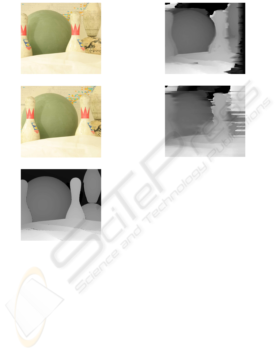
(a) right image
(b) left image
(c) disparity map of right image
Figure 3: Two stereo images and the corresponding refer-
ence disparity map.
4.1 The Hidden Markov Model
Each row of the left image is considered as a HMM.
Thus, the running variable is the row index i. The
state variable of the HMM is taken to be the dis-
parity x
i
. The set of allowable states is: x
i
∈ Ω =
{K
min
,..., K
max
}. K
min
and K
max
are the minimum
and the maximum disparities between the two im-
ages. The number of different states is K = K
max
−
K
min
+ 1. The transition probabilities between con-
secutive states are given by the transition probability
P
t
(x
i+1
= n|x
i
= m).
The disparity x
i
along an image row is a piecewise
continuous function of i. Sudden jumps are caused by
occlusions and boundaries between adjacent objects
of different depth in the scene, but for the remain-
(a) the new likelihood function
(b) NCC based likelihood
Figure 4: Reconstructed depth maps.
ing part the depth tends to be smooth. We can model
this prior knowledge by selecting P
t
(x
i+1
= n|x
i
= m)
such that the next state x
i+1
is likely to be close to the
current state x
i
. The variable has the highest probabil-
ity to stay in the same state. The probability should
decrease as the absolute difference ∆ ≡ |x
i+1
−x
i
| in-
creases. However, the probability should also allow
the large jumps that are caused by occlusions and ob-
ject boundaries.
In our experiments, P
t
consists of two modes.
Large jumps are modelled with an overall probabil-
ity P
outlier
uniformly distributed over the range x
i
−
J
max
,··· ,x
i
+J
max
. In this mode, each state within this
range is reached with a probability P
outlier
/(2J
max
+
1). Inliers are modelled with an overall probability
of 1 −P
outlier
. Here, the transition probability lin-
early decreases with ∆ up to where ∆ is larger than
a threshold T
max
. We chose P
outlier
= 0.05, J
max
= 8,
and T
max
= 3. Note, however, that the choice of P
t
could be refined by, for instance, using the uniqueness
constraint on the disparities (Faugeras, 1993).
4.2 Reconstruction
The selected rectified stereo pair is shown in Figure
3. These images are taken from (Hirschmller and
Scharstein, 2007). The scene, ’bowling1’, is chosen
because our intention is to apply the algorithm for
the reconstruction of textureless and smooth surfaces
A NEWLIKELIHOOD FUNCTION FOR STEREO MATCHING - How to Achieve Invariance to Unknown Texture, Gains
and Offsets?
607

so that later the application can be extended to the
3D reconstruction of faces. The minimum and max-
imum disparities of these images are K
min
= 374 and
K
max
= 446, which means that the state-space model
has K = 73 states.
The reconstruction is done by applying the
forward-backward algorithm to an HMM with the
transition probability described above and with the
observation probability given by eq. (7). For the cal-
culation of the likelihood expression, we consider that
the noise variance is σ
2
n
= 0.05, the gain variances
σ
2
α1
= σ
2
α1
= 0.25. We performed the calculations on
the pixels within 31x31 windows. Thus, N = 961.
The reconstruction is also performed using the
NCC as similarity measure. Since this measure is
not a probability density, it possibly should undergo
a rescaling to make it more suitable for a substitute of
the observation probability. After some experimenta-
tion, we found that the following mapping of the NCC

1
2
(1+ NCC)

γ
(18)
is a suitable choice. The best reconstruction was ob-
tained with γ = 6. We applied this expression within a
HMM with the transition probabilitydescribed above.
The windows that were used are also 31x31.
4.3 Results
The reconstructed disparity maps are shown in Fig-
ure 4. A comparison with the ground truth (Figure 3)
shows that the reconstruction based on the new likeli-
hood function is more accurate and more robust than
the one based on the NCC measure. The new likeli-
hood expression is better able to deal with, especially,
the steplike transitions due to occlusion. The NCC-
based result is oversmoothed, and cannot locate this
transitions accurately. Note that the large error on the
right-hand side of the disparity maps are caused by
missing data in the left image.
5 CONCLUSIONS
We have found an expression for a likelihood function
that can cope with unknown textures, uncertain gain
factors and uncertain offsets. In contrast to the classi-
cal approaches this likelihood is not based on some
arbitrary selected heuristics, but on a sound proba-
bilistic model. As such it can be used within a prob-
abilistic framework. The likelihood can be fine-tuned
by setting a limited range of allowable gain factors
rather than just any gain factor.
Using the model we were able to show that cop-
ing with unknown offsets can safely be done by nor-
malizing the means of the data, as done in other ap-
proaches such as the normalized correlation coeffi-
cient. Unknown gain factors and unknown textures
are dealt with in a way that differs a lot from other
approaches. Yet, the computational complexity of
the proposed metric is quite comparable with, for in-
stance, the computational load of the NCC.
We demonstrated stereo reconstruction within the
probabilistic framework by the forward-backward al-
gorithm with a suitably chosen HMM and showed
that it is a resourceful approach. We showed that
the newly proposed likelihood is more suitable for
stereo reconstruction within the probabilistic frame-
work than the NCC. The reconstruction using the
new likelihood deals better with occlusion, while the
NCC tends to oversmooth the area with greater abrupt
change in depth.
REFERENCES
Belhumeur, P. N. (1996). A bayesian approach to binocular
stereopsis. Int. J. Comput. Vision, 19(3):237–260.
Cox, I. J., Hingorani, S. L., Rao, S. B., and Maggs, B. M.
(1996). A maximum likelihood stereo algorithm.
Comput. Vis. Image Underst., 63(3):542–567.
Egnal, G. (2000). mutual information as a stereo correspon-
dence measure. Technical Report Technical Report
MS-CIS-00-20, Comp. and Inf. Science, U. of Penn-
sylvania.
Faugeras, O. (1993). Three-Dimensional Computer Vision
- A Geometric Viewpoint. The MIT Press.
Hirschmller, H. and Scharstein, D. (2007). Evalua-
tion of cost functions for stereo matching. In
IEEE Computer Society Conference on Computer
Vision and Pattern Recognition (CVPR 2007).
http://vision.middlebury.edu/stereo/data/.
Roy, S. and Cox, I. J. (1998). A maximum-flow formula-
tion of the n-camera stereo correspondence problem.
In ICCV ’98: Proceedings of the Sixth International
Conference on Computer Vision, page 492, Washing-
ton, DC, USA. IEEE Computer Society.
Spreeuwers, L. (2008). Multi-view passive acquisition
device for 3d face recognition. In BIOSIG 2008:
Biometrik und elektronische Signaturen.
van der Heijden, F., Duin, R., de Ridder, D., and Tax,
D. (2004). Classification, Parameter Estimation and
State Estimation An Engineering Approach Using
MATLAB. WILEY.
VISAPP 2009 - International Conference on Computer Vision Theory and Applications
608