BRAIN ACTIVITY DETECTION

Statistical Analysis of fMRI Data

Alicia Quir

os Carretero and Raquel Montes Diez

Departamento de Estad

ıstica e Investigaci

on Operativa, Universidad Rey Juan Carlos, M

ostoles, Madrid, Spain

Keywords:

Bayesian inference, fMRI, Activity detection, GMRF.

Abstract:

We are concerned with modelling and analysing fMRI data. An fMRI experiment is a series of images obtained

over time under two different conditions, in which regions of activity are detected by observing differences

in blood magnetism due to hemodynamic response. In this paper we propose a spatiotemporal model for

detecting brain activity in fMRI. The model makes no assumptions about the shape or form of activated

areas, except that they emit higher signals in response to a stimulus than non-activated areas do, and that

they form connected regions. The Bayesian spatial prior distributions provide a framework for detecting

active regions much as a neurologist might; based on posterior evidence over a wide range of spatial scales,

simultaneously considering the level of the voxel magnitudes together with the size of the activated area.

A single spatiotemporal Bayesian model allows more information to be obtained about the corresponding

magnetic resonance study. Despite higher computational cost, a spatiotemporal model improves the inference

ability since it takes into account the uncertainty in both the spatial and the temporal dimension. A simulated

study is used to test the model applicability and sensitivity.

1 INTRODUCTION

Magnetic Resonance Imaging is a method used to vi-

sualise the inside of living organisms as well as to de-

tect the amount of bound water in geological struc-

tures. It does not require painful interventions and it

is a widely used tool in medical diagnosis support.

The fundamental research to develop magnetic reso-

nance imaging techniques started at the beginning of

XIX century although the image obtaining technology

could not be developed until the appearance of high

speed computers. The sensitivity of Magnetic Res-

onance to changes in blood oxygen level was discov-

ered at the beginning of the 80’s and this was the great

advance that caused the advent of functional Mag-

netic Resonance Imaging. As it was already known

that changes in blood ﬂow and blood oxygenation

(collectively known as hemodynamics) in the brain

are closely linked to neural activity, fMRI could be

used from then on to track physiological activity. Im-

age acquisition with BOLD (Blood Oxygen Level De-

pendency) contrast is based on that principle (Ogawa

et al., 1990). Since 1990, fMRI has greatly increased

knowledge of the brain functions in neuroscience and,

in other ﬁelds, has contributed to a better understand-

ing of the physiology of different organs. Scientists

use fMRI to identify changes in the brain activity of

patients with certain pathologies in order to develop

new and more effective treatments and therapies. It

also serves as a guide to surgeons during operations

for the pain to be minimised.

To understand the fMRI acquisition process it

is necessary to understand the underlying physics

(Huang, 1999; Jezzard et al., 2001). Essentially, mag-

netic resonance machines build the image analysing

structural changes in an electromagnetic wave sent to

hydrogen atom protons in the different tissues of the

human body. The grey level of each voxel in the im-

age corresponds to the behaviour of a large number of

protons and it permits the identiﬁcation of different

tissues through the deﬁnition of the image contrast.

Once generated, magnetic resonance images are

digitally treated to improve quality and to minimise

error sources that could bias future statistical analy-

434

Quirós Carretero A. and Montes Diez R. (2009).

BRAIN ACTIVITY DETECTION - Statistical Analysis of fMRI Data.

In Proceedings of the Inter national Conference on Bio-inspired Systems and Signal Processing, pages 434-439

DOI: 10.5220/0001781204340439

 SciTePress

sis. Image pre-processing steps are usually: realign-

ment, unwrapping, coregistering, slice timing correc-

tion, low-pass ﬁltering, linear trend removal, smooth-

ing and normalisation. Statistical analysis is posterior

to pre-processing and its goal is to localise activity re-

gions in presence of noise. In a block-design fMRI

study, a large number of scans are obtained under dif-

ferent conditions (usually, rest and activity states) in

order to infer signiﬁcative differences between them.

2 APPROACHES TO ANALYSIS

OF fMRI DATA

Inference regarding brain activity in fMRI data is

commonly addressed through the GLM analysis,

(Friston et al., 1995), in which a linear dependency

of the BOLD signal and the hemodynamic response

function (HRF) is assumed.

Generally, the stimulus pattern is ﬁtted simply as

a box-shaped wave, slightly delayed, in order to ac-

count for the lapse of time between the stimulus onset

and the arrival of the blood to the activated area. This

box-shaped wave is convolved with a HRF template,

for which several kernels have been considered, in-

cluding Poisson (Friston et al., 1994), Gaussian (Fris-

ton et al., 1995) and gamma (Lange and Zeger, 1997).

The result of this analysis is a t, F or Z estimate for

each pixel. The next step is to threshold it (leading

to a multiple comparisons problem), in order to de-

cide, at a given level of signiﬁcance, which parts of

the brain are activated. The convolution approach is

attractive for its simplicity. However, it imposes se-

vere restrictions on the model.

The most popular and complete statistical package

is SPM (Friston et al., 2006), created by (Frackowiak

et al., 2004). SPM is based on GLM. Some other au-

thors ﬁt the HRF making use of GLM. As univariate

methods do not take into account the spatial structure

on data, they proposed a higher level spatial structure

modelisation (Bowman et al., 2008; Harrison et al.,

2007; Hartvig and Jensen, 2000; Gossl et al., 1999).

Multivariate methods provide an alternative to in-

dividual analysis of voxels, reducing the whole spa-

tiotemporal data set into certain multivariate compo-

nents with similar temporal characteristics. Multivari-

ate techniques applied to the analysis of fMRI data

include principal component analysis (Friston, 1994;

ostrand et al., 2006), independent component analy-

sis (Beckmann and Smith, 2004; Esposito et al., 2003;

McKeown et al., 2003; Calhoun et al., 2001; Po-

rill et al., 1999) and cluster analysis (Goutte et al.,

1999). Interpretation of results must be treated with

care when using these techniques, as there is a high

risk of data overﬁtting.

In order to make use of more complex models

and to overcome the multiple comparisons problem,

the best choice is to work in a Bayesian framework,

which also allows including prior information on the

expected location, shape and size of the activation ar-

eas. Most Bayesian approaches to the modelling of

fMRI data use Markov random ﬁelds (MRF) as prior

distributions, in order to account for the spatial struc-

ture present in the data (Holmes, 1995; Gossl et al.,

2001; Woolrich et al., 2004b). An alternative to these

priors are, for example, Laplacian priors on regression

coefﬁcients in GLM (Penny et al., 2005).

The fMRI data analysis is a problem that involves

the spatiotemporal relationship between a stimulus

or cognitive task and the cerebral response measured

with fMRI. In spite of the obvious spatiotemporal

nature of data, there are a few spatiotemporal mod-

els (Bowman, 2007; Katanoda et al., 2002; Woolrich

et al., 2004a), all of them based on convolution.

3 THE MODEL

We propose a spatiotemporal model to analyse fMRI

data in order to detect activity regions in the brain.

We extend (Quir

os et al., 2006), a fully Bayesian two-

stage model to localise activity regions in fMRI. In

the ﬁrst stage, the observed HRF is ﬁtted, pixelwise,

by a scaled and shifted Poisson distribution curve. A

map of values for the observed activity magnitude in

each pixel is obtained during this stage. The second

part consists of a spatial analysis of this map by the

means of a statistical model in the form of a product of

MRF. The goal of those ﬁelds is to set restrictions on

the activity patterns smoothness as prior information.

The formulation of the model is made in a simple and

natural way thanks to a small number of parameters.

Besides, the Bayesian approach provides the model of

adaptability to fMRI data and makes it efﬁcient.

The extension of this model by a single spatiotem-

poral Bayesian model allows us to obtain more in-

formation regarding the corresponding magnetic reso-

nance study. In spite of the higher computational cost,

a spatiotemporal model improves the inference ability

since it takes into account the uncertainty in both the

spatial and the temporal dimension.

3.1 The Hemodynamic Response

Function

The archetypical HRF (see ﬁgure 1) describes the lo-

cal response to the oxygen utilisation (by nerve cells)

BRAIN ACTIVITY DETECTION - Statistical Analysis of fMRI Data

435

Figure 1: Archetypical hemodynamic response curve.

and it consists of an increase in blood ﬂow to re-

gions of increased neural activity, occurring after a

delay of approximately 1-5 seconds. This hemody-

namic response rises to a peak over 4-8 seconds, be-

fore falling back to the baseline (and typically under-

shooting slightly). This leads to local changes in the

relative concentration of oxyhaemoglobin and deoxy-

haemoglobin and changes in local cerebral blood vol-

ume in addition to this change in local cerebral blood

ﬂow. This delayed response is characterized by h(τ),

where τ is the time since activity started.

Here we adopt the Poisson curve proposal (Friston

et al., 1994) and we model the HRF, for each pixel s,

by a scaled and shifted Poisson distribution density

function with mean d

, that is, a potential increase of

signal and a subsequent exponential decay,

(τ) =

(

τ−1

−d

(τ−1)!

τ = 1, 2, . .. , T − 1

0 τ = 0

where x

∈ [0, ∞] and d

∈ [0, T − 1]. Consequently,

parameter d can be interpreted as the delay of the re-

sponse with respect to the stimulus onset and x as a

measure of the magnitude of response.

3.2 Model Description

We consider a 2-dimensional block-design fMRI

study. Two consecutive blocks (a stimulation and a

resting block) are called a cycle, i.e., each cycle is

composed by T images, half of which are taken when

the stimulus is on and half when the stimulus is off.

Let y = {y

s,τ

: s = 1, . .. , N × M;τ = 0, . . . , T − 1}

be the mean of the observed hemodynamic response

curves to the stimulus paradigm. The set y plays the

role of data in our model (we take the mean to allevi-

ate the computational burden).

As the spatiotemporal model, we propose the fol-

lowing expression:

s,τ

= z



τ−1

−d

(τ − 1)!

+ ε

s,τ



+ k

+ ε

s,τ

where k is the set of basal values for each pixel that

we estimate from the mean of the ﬁrst images in the

experiment (acquired when the stimulus is off).

We consider z = {z

: s = 1, . . . , N ×M} to be a bi-

nary random ﬁeld that indicates the activity presence

or absence for each pixel of the image. To incorpo-

rate spatial connectedness (expected from activity),

we deﬁne z from thresholding of a continuous ﬁeld,

w, i.e., z

= I

>0}

for s = 1, . . ., N × M.

The error in the activity estimation and in the basal

values are, respectively, ε

s,τ

and ε

s,τ

, for which we

assume the distributions

s,τ

∼ N (0, η

s,τ

∼ N (0, σ

s,τ

Assuming independence between variables and that

s,τ

= σ

and η

s,τ

= η

, we obtain

s,τ

∼ N



τ−1

−d

(τ − 1)!

+ k

, z

+ η



3.3 Prior Distributions

When image analysis problems are treated under a

Bayesian perspective, it is necessary to formulate a

prior distribution for the image of interest, in this case,

the x ﬁeld and the generator ﬁeld of z, w. MRF are an

adequate tool for this purpose as they deﬁne expected

characteristics of the image as, for example, smooth-

ness and connection between regions (Winkler, 2003).

Making use of MRF as prior distributions for the

image of interest, activity location in a pixel is deter-

mined by its response magnitude and also by the ac-

tivity evidence in its neighbouring pixels. That is, we

establish, a priori, the expectation that activity takes

the form of regions made up of several neighbouring

pixels, penalising activity presence in isolated pixels.

Additionally, MRF can be considered as smoothing

kernels and therefore, its use as prior distributions let

us dispense with data smoothing process during the

pre-process.

The prior distribution for w is an intrinsic Gaus-

sian Markov Random Field (Rue and Held, 2005) of

ﬁrst order:

π(w) ∝ exp{−

∑

s∼t

− w

)

}. (1)

The prior distribution for w is improper as it corre-

sponds to the bidimensional generalization of a ran-

dom walk. Combining it with the likelihood, marginal

distribution for each w

becomes proper. The advan-

tage of using an intrinsic form for w is that there is

no need to specify a priori the proportion of activated

pixels.

Following the proposal of (Kornak, 2000), we de-

scribe the x–ﬁeld by the means of the natural log-

arithm of a proper Gaussian Markov Random Field

BIOSIGNALS 2009 - International Conference on Bio-inspired Systems and Signal Processing

436

(Rue and Held, 2005), i.e.:

log(x) ∼ N M V (µ1, κ

(I − βN)

−1

), (2)

where N = (n

i j

)

i, j=1,...,N×M

and n

i j

= 1 if pixels i and

j are neighbours and n

i j

= 0, otherwise. The mean

parameter µ controls the mean level of the response

magnitude, κ

controls the spatial smoothness of the

response level and β models the strength of inﬂuence

that neighbouring pixel values have on each other rel-

ative to that of the ﬁeld’s global mean level µ.

For µ and κ

we take conjugate prior distributions:

µ ∼ N (µ

, σ

∼ GI(a

, b

but with large variances, to make them be almost non

informative.

In the case of β parameter a conjugate prior distri-

bution does not exist and therefore, given the ﬂexibil-

ity of Beta distribution, we propose:

4β ∼ Be(p, q)

and hence, β ∈ [0, 0.25].

Prior distributions for the rest of parameters and

hyperparameters are:

π(d) ∼ N (µ

, σ

)

π(σ

) ∼ GI (a

, b

)

π(η

) ∼ GI (a

, b

)

We obtain the posterior distribution combin-

ing prior information with the likelihood under a

Bayesian approach. Given the model’s complexity, to

make inference over the parameters we use MCMC

methods (Gilks et al., 1996).

4 RESULTS

To test the model applicability and sensitivity, we use

a fMRI data simulation. We created this simulated

study from a real fMRI rest study made in the Ru-

ber Internacional hospital with a 3T machine. We

selected a central slice and we convolved it with an

activation pattern. This activation pattern takes the

shape of a gamma distribution in the temporal dimen-

sion and of different geometric ﬁgures to model spa-

tial activation regions. The result is a series of bidi-

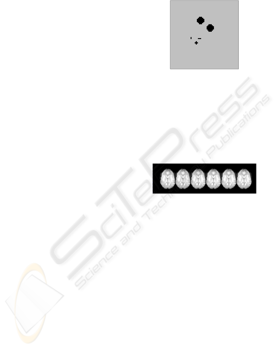
mensional slices N × M = 64 × 64 pixels. Figure 2

shows the phantom that we use to simulate the activ-

ity. Pixels of different regions have different signal

intensity (1% and 2% of the signal). The simulated

study resembles a block-design experiment with 70

scans: 3 cycles of T = 20 images each plus a rest pe-

riod at the beginning of the experiment (to calculate

Figure 2: Activity phantom used to simulate the response

paradigm to an stimulus in the simulated study.

k, the baseline value for each pixel map). In each cy-

cle, the ﬁrst ten images are taken while the stimulus

is on and the last ten images when it ceases. Figure 3

shows several slices of the simulated study. Some of

them are taken during the rest period and some dur-

ing the activity period. We observe that, to the human

eye, there are no notable differences between them,

and consequently it is not possible to discriminate ac-

tivity regions at sight.

Figure 3: Several slices of the study.

Using MCMC methods, we obtained a total of

12000 samples, 4000 of which were discarded as

burn-in. Subsequently, 8000 samples were used for

posterior inference.

In the temporal dimension, we observe for each

pixel how the hemodynamic response curve is ﬁtted

by a Poisson distribution of parameter d

, multiplied

by a scale factor (for the curve to reach the response

magnitude), x

. Figure 4 shows the ﬁtting for one of

the active pixels. It can be appreciated that the em-

pirical curve (in black) is essentially noisy and that it

adopt the archetypical shape of the hemodynamic re-

sponse described above. In the same ﬁgure, the red

curve corresponds to the Poisson curve that ﬁts the

empirical one.

In the spatial dimension, we obtained results in re-

lation to the activation regions’ shape together with its

magnitude. The z–ﬁeld posterior mean map provides

us, for each pixel, of the posterior probability of acti-

vation.

Figure 5 shows how the model is sensitive to con-

nected activation regions, rejecting posible activation

in isolated pixels, as a neurologist might judge. This

is achieved thanks to the z–ﬁeld construction from a

BRAIN ACTIVITY DETECTION - Statistical Analysis of fMRI Data

437

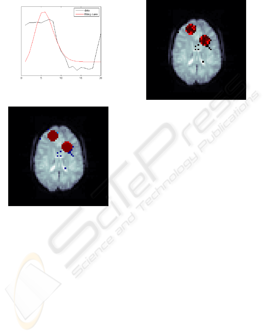
Figure 4: Hemodynamic response curve ﬁt in an active

pixel.

Figure 5: z–ﬁeld posterior mean map.

continuous ﬁeld w, whose prior distribution is a MRF,

that favours this kind of regions.

Finally, ﬁgure 6 shows the result of multiplying

pixel by pixel the z and the x ﬁelds, obtaining a mag-

nitude of activation “image” in those activated areas.

5 DISCUSSION

The Bayesian model developed here incorporates spa-

tial restrictions in order to estimate response patterns

to stimulus in fMRI experiments using MRF as prior

distributions. These MRF act as two-level spatial

smoothing ﬁlters: parameter estimation in the x–ﬁeld

(the classical level) and pixel activity identifying in

the z–ﬁeld. This smoothing process is made taking

into account the information provided by the neigh-

bours of a pixel, apart from the pixel value itself.

In addition, including temporal information into

the spatial model (forming a spatiotemporal model),

a source of information that other models do not take

Figure 6: Active regions magnitude of activation map, xz.

into account is incorporated, without a signiﬁcant in-

crease of computational cost in our model. This

would permit improvement of the model in the future,

for example, extending the model to all data (and not

only to the mean with respect to cycles), including the

baseline ﬁeld, k, as another parameter (instead of es-

timating it beforehand) and integrating the model into

a graphical interface.

ACKNOWLEDGEMENTS

The authors would like to thank ﬁnancial support

of the following projects TEC2006-13966-C03-01,

MTM2006-14961-C05-05 and TSI2007-66706-C04-

01 .

REFERENCES

Beckmann, C. F. and Smith, S. M. (2004). Probabilistic

independent component analysis for functional mag-

netic resonance imaging. IEEE Transactions on Med-

ical Imaging, 23(2):137–152.

Bowman, F. D. (2007). Spatiotemporal models for re-

gion of interest analysis of functional neuroimaging

data. Journal of the American Statistical Association,

102(478):442–453.

Bowman, F. D., Caffo, B. S., Bassett, S. S., and Kilts, C.

(2008). A bayesian hierarchical framework for spatial

modeling of fmri data. NeuroImage, 39(1):146–156.

Calhoun, V. D., Adali, T., McGinty, V. B., Pekar, J. J., Wat-

son, T. D., and Pearlson, G. D. (2001). fmri activation

in a visual-perception task: Network of areas detected

using the general linear model and independent com-

ponents analysis. NeuroImage, 14(5):1080–1088.

Esposito, F., Seifritz, E., Formisano, E., Morrone, R., Scara-

bino, T., Tedeschi, G., Cirillo, S., Goebel, R., and

BIOSIGNALS 2009 - International Conference on Bio-inspired Systems and Signal Processing

438

Di Salle, F. (2003). Real-time independent com-

ponent analysis of fmri time-series. NeuroImage,

20(4):2209–2224.

Frackowiak, R. S. J., Friston, K. J., Frith, C. D., Dolan,

R. J., Price, C. J., Zeki, S., Ashburner, J. T., and Penny,

W. D. (2004). Human Brain Function. Academic

Press.

Friston, K. J. (1994). Functional and effective connectivity

in neuroimaging: A synthesis. Human Brain Map-

ping, 2:56–78.

Friston, K. J., Ashburner, J., Kiebel, S., Nichols, T., and

Penny, W. (2006). Statistical Parametric Mapping:

The Analysis of Functional Brain Images. Elsevier,

London.

Friston, K. J., Holmes, A. P., Poline, J., Gransby, P. J.,

Williams, S. C. R., Frackowiak, J., R. S., and Turner,

R. (1995). Analysis of fmri time - series revisited.

NeuroImage, 2(1):45–53.

Friston, K. J., Jezzard, P., and Turner, R. (1994). Analysis

of functional mri time-series. Human Brain Mapping,

1(2):153–171.

Gilks, W. R., Richardson, S., and Spiegelhalter, D. J.

(1996). Markov Chain Monte Carlo in Practice.

Chapman & Hall/CRC.

Gossl, C., Auer, D. P., and Fahrmeir, L. (1999). A bayesian

approach for spatial connectivity in fmri. Poster No.

483 Biometrics, 57:554–562.

Gossl, C., Auer, D. P., and Fahrmeir, L. (2001). Bayesian

spatiotemporal inference in functional magnetic reso-

nance imaging. Biometrics, 57(2):554–562.

Goutte, C., Toft, P., Rostrup, E., Nielsen, F. A., and Hansen,

L. K. (1999). On clustering fmri time series. Neu-

roImage, 9(3):298–310.

Harrison, L. M., Penny, W., Ashburner, J., Trujillo-Barreto,

N., and Friston, K. J. (2007). Diffusion-based spatial

priors for imaging. NeuroImage, 38(4):677–695.

Hartvig, N. and Jensen, J. (2000). Spatial mixture

modelling of fmri data. Human Brain Mapping,

11(4):233–248.

Holmes, A. (1995). Statistical Issues in Functional Brain

Mapping. Chapter 5 – An Empirical Bayesian Ap-

proach. PhD thesis.

Huang, H. (1999). PACS: basic principles and applications.

Wiley-Liss, New York.

Jezzard, P., Matthews, P. M., and Smith, S. M. (2001).

Functional MRI: An introduction to methods. Oxford

University Press, New York.

Katanoda, K., Matsuda, Y., and Sugishita, M. (2002). A

spatio-temporal regression model for the analysis of

functional mri data. NeuroImage, 17(3):1415–1428.

Kornak, J. (2000). Bayesian Spatial Inference from Haemo-

dynamic Response Parameters in Functional Mag-

netic Resonance Imaging. PhD thesis, University of

Nottingham.

Lange, N. and Zeger, S. L. (1997). Non - linear fourier

time series analysis for human brain mapping by func-

tional magnetic resonance imaging. Applied Statistics,

46(1):1–29.

McKeown, M. J., Hansen, L. K., , and Sejnowsk, T. J.

(2003). Independent component analysis of functional

mri: what is signal and what is noise? Current Opin-

ion in Neurobiology, 13(5):620–629.

Ogawa, S., Lee, T. M., Kay, A. R., and Tank, D. W. (1990).

Brain magnetic resonance imaging with contrast de-

pendent on blood oxygenation. Proceedings of the

National Academy of Sciences of the United States of

America, 87(24):9868–9872.

Penny, W. D., Trujilllo-Barreto, N. J., and Friston, K. J.

(2005). Bayesian fmri time series analysis with spatial

priors. NeuroImage, 24(2):350–362.

Porill, J., Stone, J. V., Mayhew, J. E. W., Berwick, J., and

Coffey, P. (1999). Spatio - temporal data analysis us-

ing weak linear models. In Mardia, K., otro, and otro,

editors, Spatial Temporal Modelling and its Applica-

tions, pages 17–20.

Quir

os, A., Montes, R., and Hernandez, J. (2006). A fully

bayesian two - stage model for detecting brain ac-

tivity in fmri. Lecture Notes in Computer Science,

4345:334–345.

Rue, H. and Held, L. (2005). Gaussian Markov Ran-

dom Fields: Theory and Applications, volume 104

of Monographs on Statistics and Applied Probability.

Chapman & Hall/CRC, London.

ostrand, K., Lund, T. E., Madsen, K. H., and Larsen,

R. (2006). Sparse PCA, a new method for unsuper-

vised analyses of fmri data. In Proc. International So-

ciety of Magnetic Resonance In Medicine - ISMRM

2006, Seattle, Washington, USA, Berkeley, CA, USA.

ISMRM.

Winkler, G. (2003). Image Analysis, Random Fields and

Markov Chain Monte Carlo Methods. A Mathematical

Introduction. Springer, cop.

Woolrich, M. W., Behrens, T. E. J., and Smith, S. M.

(2004a). Constrained linear basis sets for hrf

modelling using variational bayes. NeuroImage,

21(4):1748–1761.

Woolrich, M. W., Jenkinson, M., Brady, J. M., and Smith,

S. M. (2004b). Fully bayesian spatio - temporal mod-

eling of fmri data. IEEE Transactions on Medical

Imaging, 23(2):213–231.

BRAIN ACTIVITY DETECTION - Statistical Analysis of fMRI Data

439