
THE PULL-PUSH ALGORITHM REVISITED
Improvements, Computation of Point Densities, and GPU Implementation
Martin Kraus
Computer Graphics & Visualization Group, Technische Universit¨at M¨unchen, Boltzmannstraße 3, 85748 Garching, Germany
Keywords:
Pyramid algorithm, Image processing, Real-time rendering, Scattered data, Meshless data, Interpolation, GPU.
Abstract:
The pull-push algorithm is a well-known and very efficient pyramid algorithm for the interpolation of scattered
data with many applications in computer graphics. However, the original algorithm is not very well suited for
an implementation on GPUs (graphics processing units). In this work, several improvements of the algorithm
are presented to overcome this limitation, and important details of the algorithm are clarified, in particular the
importance of the correct normalization of the employed filters. Moreover, we present an extension for a very
efficient estimate of the local density of sample points.
1 INTRODUCTION
Interpolation of scattered data points is a classi-
cal problem in computer graphics with many appli-
cations, e.g., inpainting, reconstruction of smooth
functions from meshless point data, image post-
processing effects, etc. (Gortler et al., 1996; Drori
et al., 2003). As recent GPU implementations of
pyramid algorithms for scattered data interpolation
achieve real-time performances, they are also suited
for real-time rendering and real-time video processing
(Lefebvre et al., 2005; Strengert et al., 2006; Guen-
nebaud et al., 2007; Kraus and Strengert, 2007a).
However, there are particularly challenging ren-
dering algorithms, which require the interpolation of
scattered pixels for multiple images per frame. For
example, the rendering of depth-of-field effects by
Kraus and Strengert (Kraus and Strengert, 2007a) re-
quires two full-screen interpolation passes for each
“subimage” with 1 to 20 “subimages” per frame (de-
pending on the strength of the effect). Thus, even
a high-performance GPU implementation of scat-
tered data interpolation can constitute a serious per-
formance bottleneck for some rendering algorithms.
Therefore, this work is concerned with improvements
of GPU implementations of the very efficient pull-
push algorithm by Gortler et al. (Gortler et al., 1996).
The next section briefly summarizes related work
while Section 3 presents our algorithmic improve-
ments of the pull-push algorithm and compares them
to the original algorithm. Section 4 presents a variant
of the algorithm to compute the local density of sam-
ple points, and in Section 5, the GPU implementations
of the algorithms and their performance is discussed.
2 RELATED WORK
The original pull-push algorithm by Gortler et al.
(Gortler et al., 1996) is based on work by Burt (Burt,
1981; Burt, 1988) and Mitchell (Mitchell, 1987)
and was used to interpolate between many sampling
points in a four-dimensionaldomain in the Lumigraph
system.
A variant of the pull-push algorithm was em-
ployed, for example, by Drori et al. (Drori et al.,
2003) for an initial reconstruction of missing parts
of images. Lefebvre et al. (Lefebvre et al., 2005)
used a GPU-based implementation for inpainting
gaps in texture maps. Strengert et al. (Strengert et al.,
2006) proposed a more efficient GPU implementa-
tion, which is of linear time complexity in the number
of pixels. The algorithm by Strengert et al. was em-
ployed by Kraus and Strengert (Kraus and Strengert,
2007a) to disocclude pixels in their depth-of-field al-
gorithm. Guennebaud et al. (Guennebaud et al., 2007)
employed a GPU implementation of the pull-push al-
gorithm to reconstruct soft shadows from a reduced
number of sample points; however, they did not de-
scribe any details of their implementation.
179
Kraus M. (2009).
THE PULL-PUSH ALGORITHM REVISITED - Improvements, Computation of Point Densities, and GPU Implementation.
In Proceedings of the Fourth International Conference on Computer Graphics Theory and Applications, pages 179-184
DOI: 10.5220/0001772601790184
Copyright
c
SciTePress
x
n
0
x
n−1
0
x
n−1
1
...
x
2
0
...
x
2
2
n−2
−1
x
1
0
x
1
1
...
x
1
2
n−1
−2
x
1
2
n−1
−1
x
0
0
x
0
1
x
0
2
x
0
3
...
x
0
2
n
−4
x
0
2
n
−3
x
0
2
n
−2
x
0
2
n
−1
Figure 1: Illustration of the pixels x
r
i
of an image pyramid
for a one-dimensional input image x
0
i
of size 2
n
.
3 REVISION OF THE PULL-PUSH
ALGORITHM
3.1 Pull
The original pull phase by Gortler et al. (Gortler et al.,
1996) computes an image pyramid of data values x
and positive weights w using a “pull filter”
˜
h. The
input image determines the size of the finest pyramid
level r = 0 while the size of pyramid level r+1 is half
of the size of pyramid level r in each dimension. For
clarity we describe the algorithm for one-dimensional
images and restrict their sizes to powers of two. Data
values of pyramid level r are denoted by x
r
i
and their
weights by w
r
i
where r equals 0 for the original (finest)
resolution and pixels are indexed by i. This structure
of a one-dimensional image pyramid is illustrated in
Figure 1.
If the pull filter is specified by a discrete sequence
˜
h of positive numbers, Gortler et al. suggest to com-
pute the pixels of the next coarser image level by:
w
r+1
i
=
∑
k
˜
h
k−2i
min(w
r
k
, 1) (1)
x
r+1
i
=
1
w
r+1
i
∑
k
˜
h
k−2i
min(w
r
k
, 1)x
r
k
(2)
To reduce the number of clamp operations, i.e., min
functions, we propose to introduce clamped weights
ˆw
r
i
and weighted data values ˜x
r
i
, in particular for the
input data on level r = 0:
ˆw
0
i
def
= min
w
0
i
, 1
, ˜x
0
i
def
= ˆw
0
i
x
0
i
(3)
The computation of coarser image levels can now be
performed with just one clamp operation and basic
filter operations:
w
r+1
i
=
∑
k
˜
h
k−2i
ˆw
r
k
(4)
ˆw
r+1
i
= min
w
r+1
i
, 1
(5)
˜x
r+1
i
=
ˆw
r+1
i
w
r+1
i
∑
k
˜
h
k−2i
˜x
r
k
(6)
This formulation is more suited for an efficient GPU
implementation as discussed in Section 5.
It should be noted that the normalization of
˜
h is
crucial for the quality of the resulting interpolation.
As shown in Section 3.3, a normalization of the max-
imum to 1 provides good results in most cases while
a normalization of the integral of the filter
˜
h to 1 leads
to significantly worse results.
Our new formulation encapsulates the nonlinear
part of the pull phase in a single clamp operation in
Equation 5, which can be replaced easily by a contin-
uous operation. For example, one could use a filter
˜
h with a normalization such that its integral is 1 and
achieve an effect similar to the nonlinear clamp oper-
ation by employing the following equation instead of
Equation 5:
ˆw
r+1
i
= 1−
1− w
r+1
i
γ
(7)
Here, γ is a parameter that controls the range of influ-
ence of data points: larger values of γ tend to result in
larger regions around isolated data points where the
interpolated values are close to the values specified
for the data points; examples are given in Section 3.3.
3.2 Push
After the image pyramid has been computed, a se-
quence of push operations recomputes all levels from
coarse to fine with a “push filter” h. First, two tempo-
rary values are computed:
ω
r
i
=
∑
k
h
i−2k
min
w
r+1
k
, 1
(8)
χ
r
i
=
1
ω
r
i
∑
k
h
i−2k
min
w
r+1
k
, 1
x
r+1
k
(9)
Note that Gortler et al. use the symbol tw instead of ω
and tx instead of χ.
These temporary values are blended with the pre-
viously computed pyramid image. However, the
equations provided by Gortler et al. lack clamping op-
erations; the corrected equations are:
x
r
i
= χ
r
i
(1− min(w
r
k
, 1)) + min(w
r
k
, 1)x
r
i
(10)
w
r
i
= min(ω
r
i
, 1)(1− min(w
r
k
, 1))
+min(w
r
k
, 1) (11)
GRAPP 2009 - International Conference on Computer Graphics Theory and Applications
180
50 100 150 200 250
i
0.2
0.4
0.6
0.8
1
x
i
0
(a)
50 100 150 200 250
i
0.2
0.4
0.6
0.8
1
x
i
0
(b)
50 100 150 200 250
i
0.2
0.4
0.6
0.8
1
x
i
0
(c)
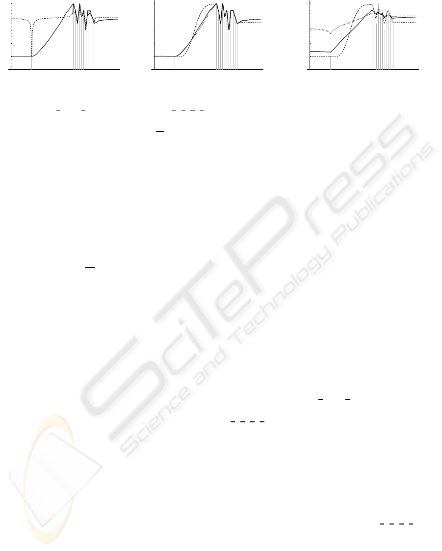
Figure 2: (a) Interpolation of a set of scattered data (gray bars) by the “original” algorithm by Gortler et al. (Gortler et al.,
1996) with
˜
h =
1
3
, 1, 1,
1
3
(solid line) and
˜
h =
1
8
,
3
8
,
3
8
,
1
8
(dashed line). (b) Interpolation by the “w/o clamp” algorithm
for γ = 4 (solid line) and γ = 16 (dashed line). For comparison, the result of the original algorithm is also included (dotted
line). (c) Same as (b) for input data of weight
1
32
instead of 1.
These equations can also be simplified by employing
clamped weights ˆw
r
i
and weighted data values ˜x
r
i
as in-
troduced in the previous section. For the push phase
we can additionally assume a normalization of the
push filter h such that no further clamp operations are
necessary. Therefore, Equations 8–11 can be rewrit-
ten as:
ˆ
ω
r
i
=
∑
k
h
i−2k
ˆw
r+1
k
(12)
χ
r
i
=
1
ˆ
ω
r
i
∑
k
h
i−2k
˜x
r+1
k
(13)
x
r
i
= χ
r
i
(1− ˆw
r
k
) + ˜x
r
i
(14)
ˆw
r
i
=
ˆ
ω
r
i
(1− ˆw
r
k
) + ˆw
r
k
(15)
˜x
r
i
= ˆw
r
i
x
r
i
(16)
These filter operations can be implemented very ef-
ficiently (see Section 5); however, the linear inter-
polation with weights ˆw
r
k
and 1 − ˆw
r
k
cannot be im-
plemented by standard blending on GPUs due to the
multiplication in Equation 16.
Fortunately, these equations can be further simpli-
fied by a new approximation, which works very well
for most input data and filters
˜
h and h. As noted
above, the pull filter
˜
h should be scaled such that
the weights ˆw
r
k
quickly approach 1 in coarser pyra-
mid levels. During the push phase these weights are
further increased, thus, they are usually equal to 1 or
close to 1 in all pyramid levels. This motivates a vari-
ation of the blending such that all new weights ˆw
r
k
are
(implicitly) set to 1. Thus, Equations 12–16 are sig-
nificantly simplified to only two equations:
χ
r
i
=
∑
k
h
i−2k
x
r+1
k
(17)
x
r
i
= χ
r
i
(1− ˆw
r
k
) + ˜x
r
i
(18)
Note that we start with x
r+1
k
instead of ˜x
r+1
k
on the
coarsest level, which can be easily computed in the
last step of the pull phase by avoiding the multiplica-
tion with ˆw
r+1
i
in Equation 6. For all but the first iter-
ation, x
r+1
k
in Equation 17 refers to the pyramid level
that was most recently computed according to Equa-
tion 18 in the push phase, while ˆw
r
k
and ˜x
r
i
in Equa-
tion 18 refer to values computed in the pull phase.
Our new formulation allows for both an efficient
GPU implementation of the filtering operations by
texture filtering as well as an efficient GPU imple-
mentation of the linear interpolation by frame buffer
blending as discussed in Section 5.
3.3 Comparison of Variants
In this section, we compare the original algorithm by
Gortler et al. (Gortler et al., 1996) with the two vari-
ants proposed in Sections 3.1 and 3.2.
3.3.1 “Original” Algorithm
For the purpose of this comparison, the “original” al-
gorithm is described by Equations 3–6 for the pull
phase and Equations 8–11 for the push phase. A
one-dimensional pull filter
˜
h is used, which is de-
fined by the sequence
1
3
, 1, 1,
1
3
, i.e., the maximum
is normalized to 1. The push filter h is defined by
1
4
,
3
4
,
3
4
,
1
4
. These filters correspond to quadratic B-
spline filters (Catmull and Clark, 1978) and are par-
ticularly well suited for GPU implementations (Kraus
and Strengert, 2007b).
Figure 2a depicts a set of scattered input pixels
of weight 1 in a one-dimensional image of dimen-
sion 256 and the data interpolation computed with
the original algorithm by Gortler et al. as described
above. For comparison, the results with a differently
normalized pull filter
˜
h specified by
1
8
,
3
8
,
3
8
,
1
8
, is
also included. With input weights less than or equal to
1, this normalization guarantees that all weights stay
less than or are equal to 1 in the pull phase, therefore,
the clamp operations are unnecessary.
However, the latter pull filter does not provide a
smooth interpolation of the input points. In fact, it ap-
pears to be extremely difficult—if not impossible—to
THE PULL-PUSH ALGORITHM REVISITED - Improvements, Computation of Point Densities, and GPU Implementation
181
(a) (b) (c)
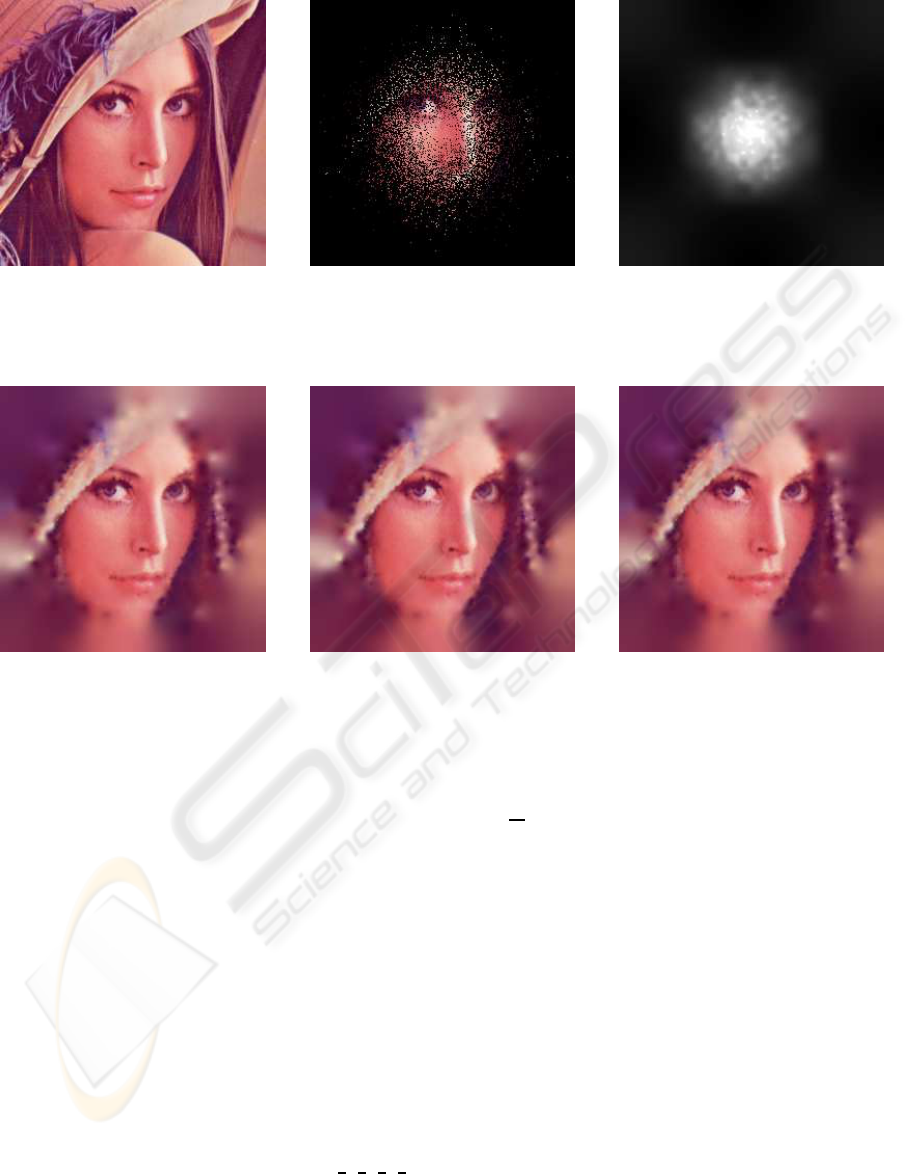
Figure 3: (a) A two-dimensional image of size 256× 256. (b) Masked variant of the image in (a): the weight of black pixels
is 0, the weight of all others is 1. (c) Density of the pixels with weight 1 computed by the algorithm presented in Section 4.
(a) (b) (c)
Figure 4: Images reconstructed from Figure 3b using (a) the “original” algorithm, (b) the “w/o clamp” variant, (c) the “w/o
weight” variant.
design appropriate pull filters for the original algo-
rithm that do not require clamping operations but still
result in smooth interpolations. Thus, in contrast to
the discussion by Gortler et al., the clamping is not
only necessary to limit the influence of clusters of
many input points but it is also crucial for a smooth
interpolation in general.
3.3.2 Variant “w/o clamp”
In order avoid the nondifferentiable clamping and
to simplify the design of pull filters, we propose
a first variant of Gortler et al.’s algorithm, named
“w/o clamp,” which replaces the clamping specified
in Equation 5 by the differentiable Equation 7. For
this variant of the algorithm, the integral of the pull
filter
˜
h has to be normalized to 1 in order to guarantee
that weights do not exceed 1. We choose
1
8
,
3
8
,
3
8
,
1
8
for the examples depicted in Figure 2b and 2c. The
parameter γ in Equation 7 was set to 4 and 16 in order
to show its influence.
While the input pixels in Figure 2b are the same
as in Figure 2a, the input weights in Figure 2c are
only
1
32
instead of 1 in Figure 2b. The dotted curve
depicted in Figure 2c suggests that it is difficult to ob-
tain a smooth curve approximating sample points with
weights less than 1 using the original algorithm. The
situation is quite similar to an unsuitable normaliza-
tion of
˜
h as the clamping operation is ineffective for
several levels in both cases. On the other hand, al-
ternative nonlinear filters such as implemented in our
variant “w/o clamp,” can provide smoother curves for
input points with weights less than 1 as illustrated by
the dashed curve in Figure 2c.
3.3.3 Variant “w/o weight”
The second variant is named “w/o weight” and imple-
ments Equations 3–6 for the pull phase; however, the
multiplication with ˆw
r+1
i
in Equation 6 is skipped for
the coarsest level in order to compute x
r+1
i
instead of
˜x
r+1
i
. For the push phase, Equations 17 and 18 are
GRAPP 2009 - International Conference on Computer Graphics Theory and Applications
182
employed. In our experiments, this variant and the
original algorithm computed very similar results al-
though the “w/o weight” variant employs a consider-
ably simplified push phase, which is better suited for
an efficient implementation on GPUs.
3.3.4 Two-Dimensional Examples
Figure 4 presents the two-dimensional results for the
input depicted in Figure 3b. Visually there are no dif-
ferences between the result of the original algorithm
employed for Figure 4a and the results for the two
new variants of the algorithm shown in Figure 4b and
Figure 4c.
4 COMPUTATION OF POINT
DENSITIES
It is often useful to compute a local density of scat-
tered points, for example in order to decide where to
place additional sampling points. Here we present a
computation of the local density of input points by a
variant of the presented pull-push algorithm.
We assume that all weights of input pixels w
0
i
are
equal to 1 and all weights of unspecified pixels are
0. In this case, the pyramid images w
r
i
computed in
the pull phase are in fact approximations of the den-
sity of input points if the integral of the pull filter
˜
h
is normalized to 1. However, it is crucial to choose
an appropriate pyramid level r. In particular, r should
be chosen locally. To this end, we base the computa-
tion of the point density on those values w
r
i
where r
is appropriate for the specific position i. This can be
achieved by introducing new weights p
r
i
for the inter-
polation of densities w
r
i
: the weight p
r
i
determines the
influence of w
r
i
analogously to the role w
r
i
played for
x
r
i
in the original pull-push algorithm.
We determine actual values for p
r
i
in dependency
of the average number ¯n
r
i
of input points at pixel i in
the pyramid image at level r:
¯n
r
i
def
= 2
r
w
r
i
(19)
If the average number of input points per pixel ¯n
r
i
is
less than 1, p
r
i
should be 0 because the correspond-
ing w
r
i
is very likely to overestimate the local density
in the neighborhood of a single, isolated input point.
On the other hand, if ¯n
r
i
is very large, p
r
i
should also
be 0 as local variations of the density of input points
are not reflected by the corresponding w
r
i
if too many
input points are included in the average. In between
these extremes, p
r
i
is set according to a function p( ¯n),
which is application-specific as even very fine local
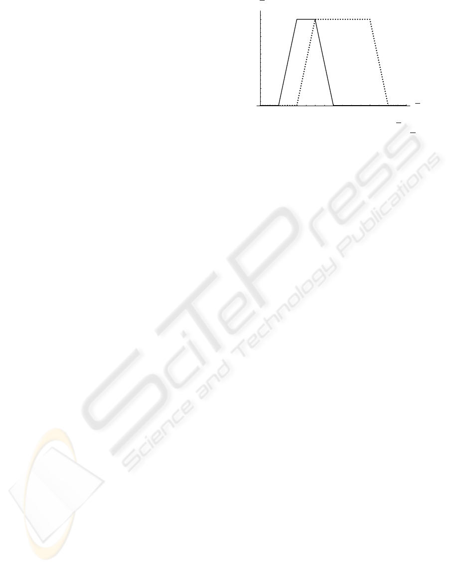
2 4 6 8
n
0.2
0.4
0.6
0.8
1
pHnL
Figure 5: Two examples for the function p(n) to deter-
mine weights depending on the average number n of in-
put points per pixel. The solid curve is suitable for one-
dimensional images while the dotted curve is suitable for
two-dimensional images.
variations are of interest in some cases—for exam-
ple when estimating the distance to the nearest in-
put point—while other applications—in particular for
high-dimensional images—require larger values of ¯n
r
i
to reliably estimate the density of input points. Fig-
ure 5 illustrates two examples for the function p( ¯n).
Having computed densities w
r
i
and their weights
p
r
i
in the pull phase, we can then apply a push phase,
which reconstructs a smooth function for w
0
i
on the
finest pyramid level analogously to reconstructing a
smooth function x
0
i
from data values x
r
i
and weights
w
r
i
. Next we describe this algorithm for the GPU-
friendly variant of the pull-push algorithm presented
in Section 3.2 (called “w/o weight” in Section 3.3).
The algorithm starts with an input image w
0
i
,
where the w
0
i
’s are either 0 or 1. The pull phase im-
plements the following equations:
w
r+1
i
=
∑
k
˜
h
k−2i
w
r
k
(20)
¯n
r+1
i
= 2
r+1
w
r+1
i
(21)
p
r+1
i
= p
¯n
r+1
i
(22)
As mentioned above, the integral of the pull filter
˜
h
has to be normalized to 1. The push filter h has to be
normalized analogously and is used in the push phase,
which recomputes the image pyramid from coarse to
fine levels using these equations:
χ
r
i
=
∑
k
h
i−2k
w
r+1
k
(23)
w
r
i
= χ
r
i
(1− p
r
k
) + p
r
k
w
r
i
(24)
The finest pyramid image w
r
i
is the resulting estimate
of the local density of points.
Figure 3c depicts the resulting density for the in-
put shown in Figure 3b. The two-dimensional gener-
alizations of the same pull and push filters were em-
ployed and the dotted curve in Figure 5 was used for
p( ¯n).
THE PULL-PUSH ALGORITHM REVISITED - Improvements, Computation of Point Densities, and GPU Implementation
183

5 GPU IMPLEMENTATION
While there are very efficient GPU implementations
of linear filtering (Kraus and Strengert, 2007b), any
additional functions in the summation (as in Equa-
tion 1) or additional nonconstant factors (as in Equa-
tion 2) defeat an efficient GPU implementation. This
problem is solved by our improvements presented in
Section 3, in particular Equations 4, 6, and 17.
For multidimensional data (e.g., RGB images) the
filtering operations in Equations 6 and 17 can be per-
formed in parallel for up to 3 components on GPUs.
Moreover, the filtering of weights in Equation 4 can
be performed in parallel in the A component of an
RGBA texture image in order to implement Equa-
tion 18 by alpha-blending. Note that only ˆw
r
i
and ˜x
r
i
have to be stored in the pull phase, while the push
phase only stores new values for x
r
i
in place of the
values ˜x
r
i
, which were computed in the pull phase.
While Gortler et al. (Gortler et al., 1996) claim
that Equations 8–11 can be implemented by standard
blending, this is unfortunately no longer true if the
computation is based on weighted variables ˜x
r
i
for
more efficient filtering. This problem is solved by the
approximation presented in Section 3.2, in particular
Equations 17 and 18.
The two-dimensional filters employed in Sec-
tion 3.3 require only four texture lookups per pixel
of the coarser level in the pull phase and one texture
lookup per pixel of the finer level in the push phase
if the filtering is implemented efficiently (Kraus and
Strengert, 2007b). As GPU implementations of the
proposed algorithms are bandwidth-limited, the arith-
metic operations do not significantly affect the per-
formance. Our implementation requires 0.60 ms for a
1024 × 1024 16-bit floating-point RGBA image on a
NVIDIA Quadro FX 5800 graphics board.
6 CONCLUSIONS
As shown in this work, the proposed algorithms for
the interpolation of scattered data points and the com-
putation of local densities of scattered points are well
suited for very efficient GPU implementations, which
could be used for real-time rendering or real-time im-
age and video processing.
The quality of the results computed by the pro-
posed algorithms depends on the choice of the pull
and push filters, the nonlinear function in Equation 7,
and the function p( ¯n) in Equation 22. Determining
suitable filters and functions for particular applica-
tions is part of future work.
REFERENCES
Burt, P. J. (1981). Fast Filter Transforms for Image Pro-
cessing. Computer Graphics and Image Processing,
16:20–51.
Burt, P. J. (1988). Moment images, polynomial fit filters,
and the problem of surface interpolation. In Pro-
ceedings of Computer Vision and Pattern Recognition,
pages 144–152.
Catmull, E. and Clark, J. (1978). Recursively Generated
B-Spline Surfaces on Arbitrary Topological Meshes.
Computer Aided Design, 10(6):350–355.
Drori, I., Cohen-Or, D., and Yeshurun, H. (2003).
Fragment-Based Image Completion. ACM Transac-
tions on Graphics, 22(3):303–312.
Gortler, S. J., Grzeszczuk, R., Szeliski, R., and Cohen, M. F.
(1996). The Lumigraph. In SIGGRAPH ’96: Pro-
ceedings of the 23rd Annual Conference on Computer
Graphics and Interactive Techniques, pages 43–54.
Guennebaud, G., Barthe, L., and Paulin, M. (2007). High-
Quality Adaptive Soft Shadow Mapping. Computer
Graphics forum (Proceedings Eurographics 2007),
26(3):525–533.
Kraus, M. and Strengert, M. (2007a). Depth-of-Field Ren-
dering by Pyramidal Image Processing. Computer
Graphics Forum (Conference Issue), 26(3):645–654.
Kraus, M. and Strengert, M. (2007b). Pyramid Filters Based
on Bilinear Interpolation. In Proceedings GRAPP
2007 (Volume GM/R), pages 21–28.
Lefebvre, S., Hornus, S., and Neyret, F. (2005). Octree Tex-
tures on the GPU. In Pharr, M., editor, GPU Gems 2,
pages 595–613.
Mitchell, D. P. (1987). Generating Antialiased Images at
Low Sampling Densities. In Proceedings of SIG-
GRAPH ’87, pages 65–72.
Strengert, M., Kraus, M., and Ertl, T. (2006). Pyramid
Methods in GPU-Based Image Processing. In Pro-
ceedings Vision, Modeling, and Visualization 2006,
pages 169–176.
GRAPP 2009 - International Conference on Computer Graphics Theory and Applications
184
