
SEGMENTATION THROUGH EDGE-LINKING
Segmentation for Video-based Driver Assistance Systems
Andreas Laika
BMW Group Forschung und Technik, Hanauer Straße 46, D-80992 M
¨
unchen, Germany
Adrian Taruttis and Walter Stechele
Lehrstuhl Integrierte Systeme, Technische Universit
¨
at M
¨
unchen, Arcisstraße 21, D-80333 M
¨
unchen, Germany
Keywords:
Segmentation, Edge linking, Driver assistance, Object recognition.
Abstract:
This work aims to develop an image segmentation method to be used in automotive driver assistance systems.
In this context it is possible to incorporate a priori knowledge from other sensors to ease the problem of local-
izing objects and to improve the results. It is however desired to produce accurate segmentations displaying
good edge localization and to have real time capabilities. An edge-segment grouping method is presented to
meet these aims. Edges of varying strength are detected initially. In various preprocessing steps edge-segments
are formed. A sparse graph is generated from those using perceptual grouping phenomena. Closed contours
are formed by solving the shortest path problem. Using test data fitting to the application domain, it is shown
that the proposed method provides more accurate results than the well-known Gradient Vector Field Snakes.
1 INTRODUCTION
Video based driver assistance systems offer the po-
tential to increase safety and driver comfort in future
automotive environments. Hence, it is necessary to
develop video processing techniques that can be im-
plemented within the constraints of automotive pro-
cessing systems. Below we present a method for the
segmentation of objects in images.
Using shape-information as a feature for classifi-
cation, or providing visual information to the driver
are possible applications for this approach. Spe-
cific requirements are important in this context: the
method should allow to integrate a priori knowledge
of the object, such as data obtained from other sen-
sors like a laser scanner. It should conceivably be able
to run in a real-time environment. Finally, accurate
segmentation results are desired, requiring the output
contour to closely fit to the object boundary. To meet
these aims we present an algorithm based on methods
for perceptual grouping of edge-segments.
2 STATE OF THE ART
According to (Gonzalez and Woods, 1987) segmenta-
tion is the partitioning of an image into its constituent
regions or into objects and background. Segmenta-
tion can be based on the detection of discontinuities,
based on grouping similarities in color or texture or
based on other cues like motion. If the goal of the
segmentation method is to partition an image into re-
gions of similarity, many alternatives like seeded re-
gion growing or Watershed segmentation exist. Those
techniques are relatively good at their stated goal of
segmenting images into homogeneous regions, but
the goal of this work, namely segmenting complete
objects, would require an augmentation with some ad-
ditional method for grouping regions. Fundamental
to the problem of segmenting an object is the ques-
tion of how that object is defined. Motion cannot be
used as a cue in the general case (e.g. when object and
background have the same relative velocity). Also, an
object is not necessarily homogeneous in color or tex-
ture. This leaves segmentation based on the object’s
saliency, i.e. how much an object stands out from its
background. Additionally in our case we assume the
presence of a region of interest (ROI) containing con-
tain exactly one object. Section 3.1 explains how such
43
Laika A., Taruttis A. and Stechele W. (2009).
SEGMENTATION THROUGH EDGE-LINKING - Segmentation for Video-based Driver Assistance Systems.
In Proceedings of the First International Conference on Computer Imaging Theory and Applications, pages 43-49
DOI: 10.5220/0001770700430049
Copyright
c
SciTePress

a ROI can be determined. While there is no quan-
tative definition of saliency, it is often considered in
terms of the principles of perceptual organization and
the laws of Gestalt psychology (Lowe, 1985). Ele-
ments are grouped together according to the phenom-
ena of Proximity, Similarity, Closure, Continuation,
Symmetry and Familiarity. Since many of the group-
ing phenomena found to be important in human visual
perception are related to discontinuities, an approach
to object segmentation based on edge detection is ap-
propriate.
Attempts at object segmentation based on grouping
of edge-segments (Elder and Zucker, 1996; Kiranyaz
et al., 2006; Wang et al., 2005; Stahl and Wang,
2007; Mahamud et al., 2003) roughly follow these
steps: First the input images are preprocessed before
running an edge detection algorithm over them, the
resulting edge maps are traced into edge-segments,
these edge-segments are further processed. Finally, a
search algorithm is applied to graph representations of
the edge-segments to find closed contours. Some pro-
cessing steps of our method are inspired by a related
method by Ferreira, Kiranyaz, and Gabbouj (hence-
forth referred to as FKG) (Kiranyaz et al., 2006),
which in turn,has some similarities to a method by
Elder and Zucker (Elder and Zucker, 1996).
3 THE ALGORITHM
3.1 Preprocessing
Reduction to the Region of Interest (ROI). The
method starts by reducing the image to the region
of interest (ROI). Only that part of the image is
processed further. Knowledge of that ROI can ei-
ther be generated by manually labelling or by using
additional sensors like laser-scanners or PMD 3D-
cameras. They provide information about the distance
to the object, allowing a discrimination of object and
background. Then again those sensor usually have
a much lower spatial resolution. So usually only a
bounding box of the object’s position can be deter-
mined. At best a rough contour of the object at a much
lower resolution can be found.
3.2 Prominence-Map Generation
Detection of Weak and Strong Edges. In a first
step edges of different strength are detected. The one
approach is to detect edges in different scales of a
scale space. However due to gaussian filtering edges
can move . FKG uses a cascade of bilateral filters to
Figure 1: Edge maps generated with 4 different thresholds
(top) and the corresponding Prominence map (bottom).
overcome this problem, but Runtime is high and pa-
rameters are heavily dependent on the object in the
image. We generate edge maps with different levels
of detail by increasing the edge detection thresholds
of the Canny Edge Detector (Canny, 1986) in k iter-
ations. This can be viewed as an approximate dis-
cretization of edge pixel strengths.
Combining Edges to a Prominence Map. Edge
maps are then merged into a single prominence map.
Each edge pixel i
x,y
is assigned a prominence value
p
x,y
∈
{
1,...,k
}
corresponding to the k increasing
Canny edge detection thresholds after which that edge
pixel still remains detected as an edge. Figure 1 shows
the prominence map generated from combining edge
maps with 4 different thresholds.
Morphological Thinning. Since Canny edge de-
tection does not guarantee edge-segments with a
thickness of exactly one pixel, a thinning process is
applied to the prominence map to reduce that thick-
ness to one pixel. This simplifies the subsequent edge
tracing process.
The Use of A Priori Knowledge. If additionally to
the bounding box also a rough contour of the object is
available, this is used as additional a priori knowledge
to boost the segmentation process in two ways: First
the prominence values of edge pixels in a region on
and near the contour of that mask can be increased
and are so more likely to be incorporated in the final
contour. Second the search space can be reduced by
discarding pixels which are not in that region.
3.3 Generating a Graph Representation
Tracing of Edge-segments. The process of tracing
is the first step in the transition from individual edge
pixels on the prominence map to a graph represen-
tation. To generate a list of edge-segments ES
j
∈
IMAGAPP 2009 - International Conference on Imaging Theory and Applications
44
{
ES
1
,ES
2
,...,ES
n
}
. all edges in the prominence map
are traced.An edge-segment containing a set of L 8-
connected pixels is denoted as ES
j
=
{
i
1
,i
2
,...,i
L
}
.
The two pixels with exactly one neighbor are marked
as endpoints. Pixels with two neighbors are marked as
transitional pixels. A pixel with more than two neigh-
bors is an endpoint at a junction between two or more
edge-segments. In this case one connected edge in the
prominence map is split into several edge-segments.
The prominence values corresponding to the edge
pixels are summed up to compute a prominence value
for the whole segment P
j
:
P
j
=
∑
i
x,y
∈ES
j
p
x,y
(1)
This grouping of edge pixels can be viewed as
an incorporation of the perceptual organization phe-
nomenon of proximity on the low level of edge pix-
els. edge-segments consisting of less than 3 pixels are
discarded as noise. If the tracing finds contours which
are already closed, they are stored for later considera-
tion as candidate objects (see in 3.5).
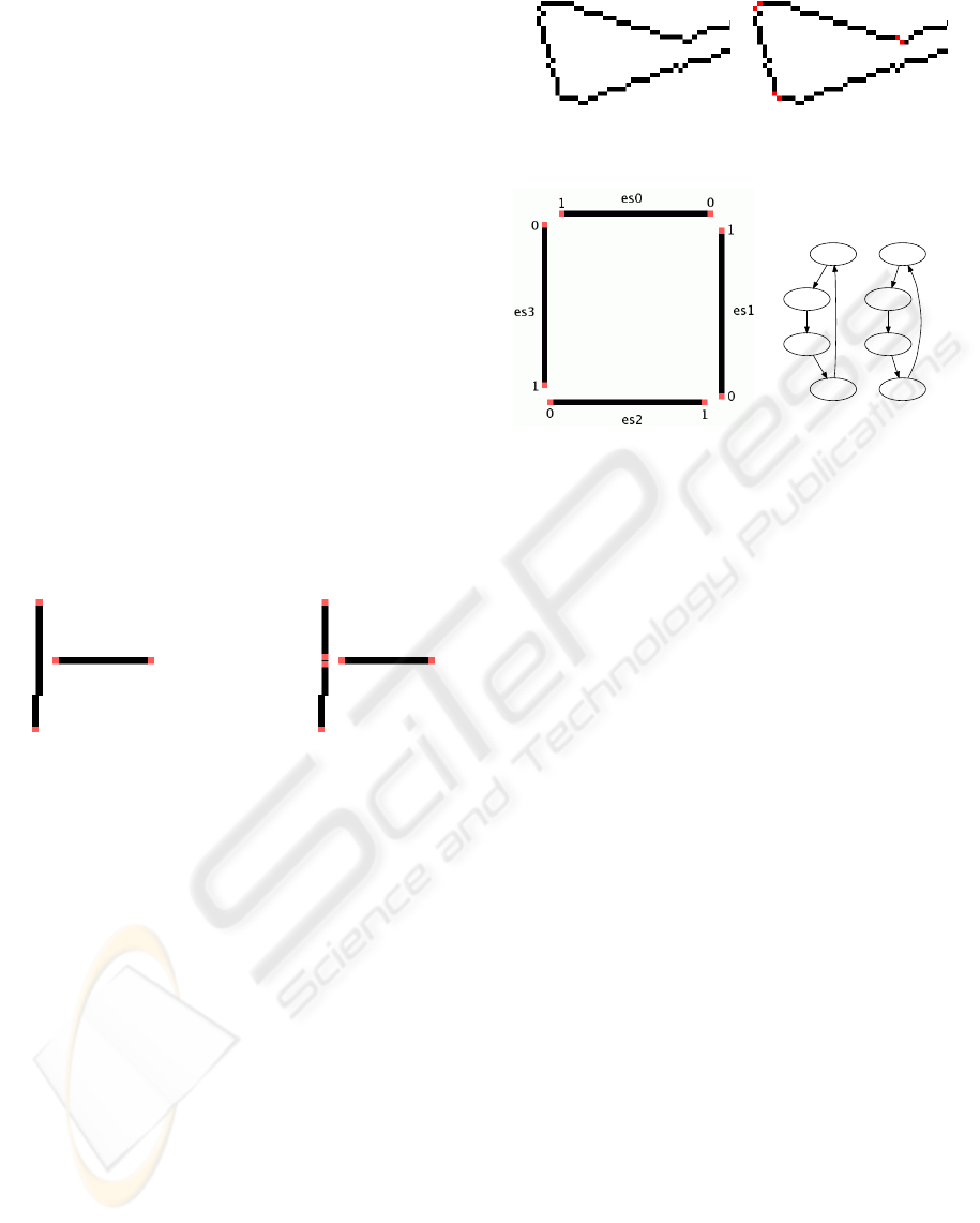
Figure 2: Junction splitting (endpoints marked in red).
Left: before, Right: after.
Junction Splitting. Figure 2 shows an edge-
segment endpoint in close proximity to a second edge-
segment. It is possible that such a configuration rep-
resents the junction of three separate edge-segments.
In order to later consider each possible grouping at
such a junction, the continuous edge must be split at
the pixel closest to the existing endpoint.
Curve Splitting. As a further step in allowing many
possible groupings of edge-segments, edge segments
with curves are split iteratively until their deviation
from the straight line joining their endpoints is be-
low a certain threshold. This splitting process follows
from the grouping phenomenon of continuation. Fig-
ure 3 shows an example image section where a curved
edge-segment is split into multiple straighter edge-
segments.
Prominence Filter. In order to reduce runtime the
number of edge-segments is reduced to the N edge-
segments with the highest prominence values P
i
.
Other edge segments are discarded.
Figure 3: Curve splitting (endpoints marked in red).
Left: before; Right: after.
es0_d0
es1_d0
es2_d0
es3_d0
es3_d1
es2_d1
es1_d1
es0_d1
Figure 4: Left: a simple edge map with edge-segments and
ends labeled; Right: the resulting directed graph.
Linking of Edge-segments. In the previous steps
edge-segments were modified to be suitable for a
graph representation. It is however also important
how to link those segments in a graph representation.
Linking all segments with each other is not an option,
since the resulting fully connected graph makes the
search infeasible. One solution is to limit the max-
imum Euclidean distance VLL
i, j
between two end-
points i
i
and i
j
. However this leads to a high or even
complete connectivity in regions with many small
edge-segments. Few edge-segments with longer gaps
on the other hand may only be connected sparsely or
not at all. Hence we limit the number of links or ver-
tices each of the endpoints can be connected with to
an upper bound denoted V (Elder and Zucker, 1996) .
3.4 Graph-based Search
Graph Representation. For the graph representa-
tion each edge-segment is represented by two vertices
in the graph; each vertex represents an edge-segment
with virtual links leaving from one of the two end-
points of that edge-segment, in other words: each ver-
tex represents a directed edge-segment. Each virtual
link from one directed edge-segment to another is rep-
resented by a directed edge in the graph. Figure 4
shows an example edge map and the corresponding
graph representation.
Edge Weights. For a graph search to be successful
the graph’s edges need meaningful weights W
ES
1
,ES
2
.
This should include both the prominence of the
edge-segment P
1
as well as the length of the gap
VLL. The dependence of grouping on VLL incor-
SEGMENTATION THROUGH EDGE-LINKING - Segmentation for Video-based Driver Assistance Systems
45

porates the grouping phenomenon of proximity.
The straight forward use of the quotient of both
W
ES
1
,ES
2
= VLL
1,2
/P
1
like in FKG however has
the disadvantage of implicitly including the edge-
segment’s length L
1
. If an edge-segment is split
at junctions or curvatures the total weight of the
resulting edges will differ from the initial weight.
Hence, we use the segment’s mean prominence. We
also raise VLL to a power, similar to (Stahl and Wang,
2007), to be able to favor longer or shorter gaps:
W
ES
1
,ES
2
=
VLL
α
1,2
1
L
1
P
1
(2)
Search. Subsequently, Dijkstra’s algorithm is ap-
plied to search for closed contours, starting from
each of the N remaining edge-segments. The search
for salient closed contours explicitly incorporates the
grouping phenomenon of closure into the method. Di-
jkstra’s algorithm finds the shortest path from a sin-
gle source to each vertex in the graph. For finding
a closed contour the source and destination vertices
are identical, and only the lowest cost nonzero path
from the source vertex back to itself is of interest.
Additionally, since each edge-segment is represented
by two vertices depending of the direction traveled
along the edge-segment, the algorithm must ensure
that no edge-segment is traversed more than once by
the closed contour. Thus Dijkstra’s algorithm must be
adjusted in three ways:
• Terminate when the shortest path to the destina-
tion vertex is found.
• The source/destination vertex must have its dis-
tance d set to infinity after the algorithm has
started so that it can be relaxed a second time.
• Relax a vertex only if the edge-segment associated
with is not on the current shortest path.
3.5 Postprocessing
Contour Selection. The best of the resulting closed
contours is selected according to the following
measure:
W =
A
1 +
∑
W
ES
j
,ES
j+1
β
(3)
With β < 1 so that area A of the contour dominates
the ranking.
4 EVALUATION AND RESULTS
4.1 The Test Environment
The algorithm presented was implemented in C++ us-
ing the OpenCV libraries. Unless otherwise stated
the tests were run on a Linux operating system with a
2GHz Intel Core 2 Duo Processor and 2GB of RAM.
Test Data. To generate the test-data, real road
scenes were recorded through windscreen of a car
using a high-dynamic range CMOS camera. 50 im-
ages with a resolution of 752 × 480 pixel were se-
lected from those scenes. Typical objects on and
near the road, like pedestrians or cars are depicted in
those scenes. Images were not selected depending on
whether they are easy to segment or not. Some have
much detail in the immediate background or weak
edges around the object boundary. A bounding box
was defined around the object of interest and a binary
segmentation mask was generated manually to serve
as ground truth for the evaluation. Two lower resolu-
tion masks were generated to simulate a priori knowl-
edge of the object shape from other sensor data, as
mentioned in 3.1.
Evaluation Method. To evaluate the results of the
segmentation method, the output segmentation mask
is compared to the ground truth mask of the manual
segmentation. Each pixel is considered separately to
give a measure of the similarity of the areas taken
up by each mask; standard methods from the field of
pattern recognition are applied as in (Fawcett, 2004).
If an on-pixel in the output mask corresponds to an
on-pixel in the ground truth mask, it is a true positive
(T P), else a false positive (FP). If an off-pixel in the
output corresponds to an off-pixel in the ground truth,
it is a true negative (T N), else a false negative (FN).
Those numbers are used to calculate the F-measure
according to equation 4:
F-measure =
2T P
2T P + FP + FN
(4)
A threshold value of F-measure corresponding to a
subjectively good segmentation is chosen at 0.85. The
number of segmentations with a value of F-measure
above this threshold, referred to as good segmenta-
tions, is used to obtain a measure for the comparative
accurateness of the method with a particular configu-
ration.
IMAGAPP 2009 - International Conference on Imaging Theory and Applications
46
4.2 Influence of the Algorithm’s
Parameters
The Total Number of Edge-segments. The graph-
based search accounts with 75% for most of the run-
time which is on average 260 ms per object. Hence
the parameters influencing the search are the most im-
portant in finding a trade-off between runtime and ac-
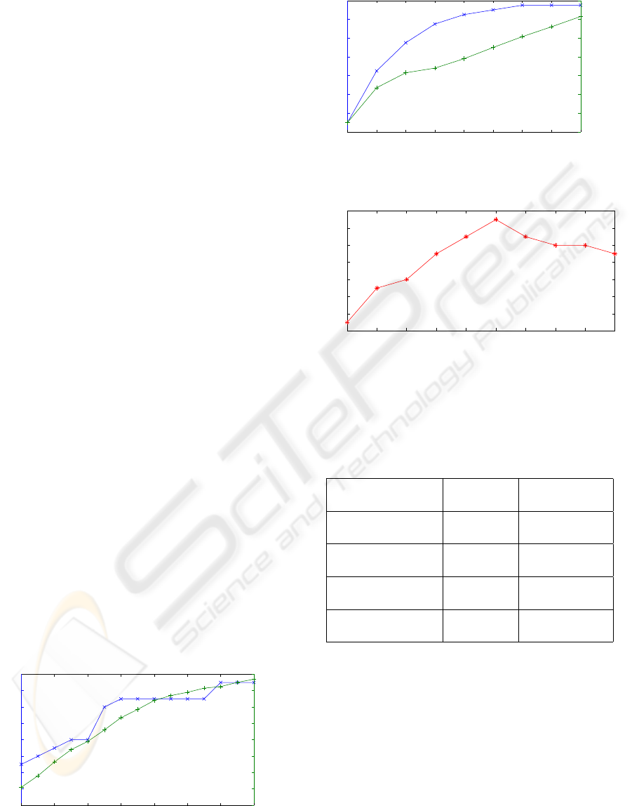
curateness. The first such parameter is the number
of edge-segments N. In figure 5 the accurateness of
the segmentations and the runtime are plotted against
N. While runtime increases continuously with just a
slight decrease towards higher values of N, accurate-
ness increases more sharply and then flattens. Choos-
ing a high accurateness per runtime suggest 160 as a
good value for N.
The Level of Connectivity of the Graph Edges.
the degree to which the graph is connected as ex-
plained in 6 the limit of nodes per vertex V is plot-
ted against accurateness of the segmentations and the
runtime. Again runtime increases continuously with
V, while accurateness increases more sharply and then
flattens out. The best accurateness per runtime ratio
is reached at values of 4 and 5, however to boost ac-
curateness a value of 7 is chosen as the default value
for subsequent experiments.
Cost Function. Figure 7 plots the segmentation ac-
curateness against α. As expected, accurateness ini-
tially rises with α as the values of VLL in the out-
put contour are reduced to a minimum to reflect the
grouping phenomenon of proximity. After α = 3.5 the
amount of good segmentations starts declining. This
value is thus a good choice which minimizes VLL and
yet still allows edge-segments with high prominence
to influence the result.
A Priori Knowledge. One of the stated aims of this
work is to present a segmentation method that allows
the integration of a priori knowledge of the object to
100 120 140 160 180 200 220 240
12
14
16
18
20
22
24
26
28
Number of edges
Accurateness − Number of good segmentations
100 120 140 160 180 200 220 240
120
140
160
180
200
220
240
260
280
Runtime (ms)
Figure 5: Number of good segmentation results and runtime
against N.
1 2 3 4 5 6 7 8 9
0
4
8
12
16
20
24
28
Number of vertices
Accurateness − Number of good segmentations
1 2 3 4 5 6 7 8 9
60
100
140
180
220
260
300
340
Runtime (ms)
Figure 6: Amount of good segmentations and runtime
against maximum successor constraint.
1 1.5 2 2.5 3 3.5 4 4.5 5 5.5
14
16
18
20
22
24
26
28
alpha
Number of good segmentations
Figure 7: Amount of good segmentations against α.
be segmented. To demonstrate the impact of a priori
knowledge of the object shape, simulated data at two
different resolutions is used as explained in 4.1. In the
Table 1: Segmentation with different A Priori Knowledge.
Shape Good Seg- Runtime
Knowledge mentations
low res - reduction 29 6.7s
of search space (58%) (134ms/Frame)
high res - reduction 38 5.5s
of search space (76%) (110ms/Frame)
high res - no reduc- 31 15.5s
tion of search space (62%) (310ms/Frame)
none 27 13.0s
(54%) (260ms/Frame)
first two tests both an increase of prominence values
and a reduction of the search space was performed.
As can be seen in Table 1 this results in a higher num-
ber of good segmentations and a reduced runtime.
Both improvements are stronger in the case of
higher resolution shape knowledge. In the third test,
only the prominence values are increased, but the
search space is not reduced. Hence, the results show
no improvement in runtime. More good segmenta-
tions are achieved than without shape knowledge, but
less as with search space reduction. In the interests
of obtaining good segmentations in short time, it is
recommended to reduce the search space to pixels in
SEGMENTATION THROUGH EDGE-LINKING - Segmentation for Video-based Driver Assistance Systems
47
the boundary region. Shape knowledge may help with
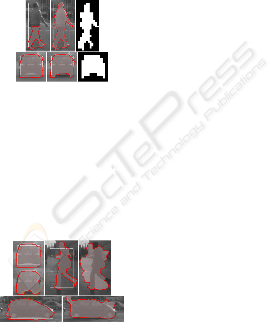
some problematic cases, like the pedestrian depicted
in Figure 8, which is cut in half due to a strong edge
at the waist.
Figure 8: Selected segmentations. Left: without shape
knowledge, Center: with higher resolution shape knowl-
edge, Right: shape masks.
4.3 Comparison with GVF Snakes
Gradient Vector Field (GVF) (Xu and Prince, 1998)
represent a well-known method with scope for us-
ing a priori knowledge of the object thus providing
a good comparison for the method proposed in this
work. The tests were conducted with a reference Mat-
lab implementation provided by the authors (Xu and
Prince, 1998) using the following parameter values:
α = 1, β = 0 and µ = 0.2. The ROIs of the proposed
method are used as initial points. With GVF Snakes,
18 (36%) good segmentations are obtained, compared
to 27 (54%) with the proposed method. In Figure 9
some segmentation results of the proposed method are
compared to segmentations from GVF Snakes. The
white boxes are the initial ROIs. In the upper left case
both methods are successful. At the bottom of the car
Figure 9: Comparison of the proposed method with GVF
Snakes. ROIs used are depicted as white boxes.
GVF Snakes perform better, since the internal forces
of the algorithm try to stick to the strong edge directly
underneath the car. However, in the other two cases
this property is problematic, since the contour there
sticks to strong edges on the background an inside the
object. In the case of the pedestrian, there are prob-
lems entering the concavities.
5 CONCLUSIONS
This work presents an approach to object-
segmentation based on the grouping of edge-
segments. In comparison with previous approaches it
introduces the following new processing steps:
Detection of weak and strong edges by increasing
edge detection thresholds provides a fast method
for ranking the prominence of detected edge pixels.
Improvement of the generation of edge-segments
by splitting at points of high curvature allows more
grouping permutations. Introduction of a new
cost-function, which allows for a trade off between
the average edge-segment prominence and edge
gap length VLL. Use of a priori knowledge to boost
segmentation results and concurrently allow for
shorter running time.
Because the closed contours are formed from edge
pixels detected by the Canny edge detector, the results
show good edge localization. The proposed method
yields better results within the problem domain of
automotive applications, than the use of GVF Snakes.
Those show more problems with background and
internal edges as well as with object concavities.
The following points outline possible directions for
further work on this topic:
Improving Contour Selection: This work also
introduces a new way to select object hypothesis
based on a formula considering both high area and
low cost. It is conceivable however, that a more
sophisticated method could be applied. It could be
either model-free as in our case or incorporation
specific knowledge of the target objects’s shape.
Using Previous Video Frames: If the method is to be
applied on video sequences, the output of a previous
frame could be used as a priori shape knowledge for
the next frame. In this case a combination and / or
comparison with motion segmentation approaches
would also be of interest.
Using Color: If colored images are available, more
salient edges could be generated with a color-edge
detector. With those, the algorithm, which would
largely remain the same, may yield better results.
IMAGAPP 2009 - International Conference on Imaging Theory and Applications
48

ACKNOWLEDGEMENTS
The authors would like to thank S.Kiranyaz et al. for
providing practical information about their method.
REFERENCES
Canny, J. (1986). A computational approach to edge de-
tection. IEEE Transactions on Pattern Analysis and
Machine Intelligence, 8(6):679–698.
Elder, J. H. and Zucker, S. W. (1996). Computing Contour
Closure. In ECCV ’96: Proceedings of the 4th Euro-
pean Conference on Computer Vision-Volume I, pages
399–412, London, UK. Springer-Verlag.
Fawcett, T. (2004). ROC Graphs: Notes and Practical Con-
siderations for Researchers. Machine Learning, 31.
Gonzalez, R. and Woods, R. (1987). Digital image process-
ing. Addison-Wesley Reading, Mass.
Kiranyaz, S., Ferreira, M., and Gabbouj, M. (2006). Auto-
matic Object Extraction over Multi-Scale Edge Field
for Multimedia Retrieval. IEEE Transactions on Im-
age Processing, 15(12):3759–3772.
Lowe, D. G. (1985). Perceptual Organization and Visual
Recognition. Kluwer Academic Publishers, Norwell,
MA, USA.
Mahamud, S., Williams, L., Thornber, K., and Xu, K.
(2003). Segmentation of multiple salient closed con-
tours from real images. IEEE Transactions on Pattern
Analysis and Machine Intelligence, 25(4):433–444.
Stahl, J. and Wang, S. (Oct. 2007). Edge Grouping Com-
bining Boundary and Region Information. Image Pro-
cessing, IEEE Transactions on, 16(10):2590–2606.
Wang, S., Kubota, T., Siskind, J. M., and Wang, J. (2005).
Salient Closed Boundary Extraction with Ratio Con-
tour. IEEE Transactions on Pattern Analysis and Ma-
chine Intelligence, 27(4):546–561.
Xu, C. and Prince, J. (1998). Snakes, shapes, and gradient
vector flow. Image Processing, IEEE Transactions on,
7(3):359–369.
SEGMENTATION THROUGH EDGE-LINKING - Segmentation for Video-based Driver Assistance Systems
49
