FOCUS OF ATTENTION AND REGION SEGREGATION BY
LOW-LEVEL GEOMETRY
J. A. Martins, J. Rodrigues and J. M. H. du Buf
Vision Laboratory, Institute for Systems and Robotics (ISR), University of the Algarve, Campus de Gambelas, 8005-139 Faro, Portugal
Keywords:
Saliency, Focus-of-Attention, Region segregation, Colour, Texture.
Abstract:
Research has shown that regions with conspicuous colours are very effective in attracting attention, and that
regions with different textures also play an important role. We present a biologically plausible model to obtain
a saliency map for Focus-of-Attention (FoA), based on colour and texture boundaries. By applying grouping
cells which are devoted to low-level geometry, boundary information can be completed such that segregated
regions are obtained. Furthermore, we show that low-level geometry, in addition to rendering filled regions,
provides important local cues like corners, bars and blobs for region categorisation. The integration of FoA,
region segregation and categorisation is important for developing fast gist vision, i.e., which types of objects
are about where in a scene.
1 INTRODUCTION
Attention of animals, also primates and humans, is
rapidly drawn towards conspicuous objects and re-
gions in the visual environment. The ability to iden-
tify such objects and regions in complex and cluttered
environments is key to survival, for locating possi-
ble prey, predators, mates or landmarks for naviga-
tion (Elazary and Itti, 2008). But attention is only one
aspect. We start to understand how our visual sys-
tem works: (1) very fast extraction of global scene
gist, (2) also fast local gist for important objects and
a rough spatial layout map, (3) in parallel with (2) the
construction of a saliency map for Focus-of-Attention
(FoA), and only then (4) sequential screening of con-
spicuous regions for precise object recognition, using
peaks and regions in the saliency map with inhibition-
of-return in order not to fixate the same region twice,
but with two strategies for FoA: first covert attention
(automatic, data-driven) possibly followed by overt
attention (consciously directed). In addition, our vi-
sual system is not analysing all information for con-
structing a complete and detailed map of our environ-
ment; it concentrates on essential information for the
task at hand and it relies on the physical environment
as external memory (Rensink, 2000).
In this paper we concentrate on three aspects: (1)
the construction of a saliency map for FoA on the ba-
sis of colour, which was shown to be very effective in
attracting attention (van de Weijer et al., 2006), also
texture (du Buf, 2007), (2) a first region segregation
by employing low-level geometry in terms of blobs,
bars and corners, and (3) using low-level geometry
allows us to reduce significantly the dimensionality
of texture features. We note that our approach is not
based on the cortical multi-scale keypoint represen-
tation as recently proposed by Rodrigues and du Buf
(2006), who built saliency maps which work verywell
for the detection of facial landmarks and for invari-
ant object recognition on homogeneous backgrounds
(Rodrigues and du Buf, 2007), but may lead to enor-
mous amounts of local peaks in natural scenes.
2 COLOUR CONSPICUITY
Colour information in a saliency map was first used
by Niebur and Koch (1996). Their model was later ex-
tended by Itti and Koch (2001), who integrated more
features, for instance intensity, edge orientation and
motion. In our approach to create a saliency model
which also contains cues for region and object segre-
gation, we therefore start by using colour information,
as this provides the most important input for attention
(van de Weijer et al., 2006), in order to build a colour
conspicuity map which will later be combined with a
texture map. But before using colour features the in-
put images must be corrected because a same object
will look different when illuminated by different light
sources, i.e., the number, power and spectra of these.
267
A. Martins J., A. Rodrigues J. and M. H. du Buf J. (2009).
FOCUS OF ATTENTION AND REGION SEGREGATION BY LOW-LEVEL GEOMETRY.
In Proceedings of the Fourth International Conference on Computer Vision Theory and Applications, pages 267-272
DOI: 10.5220/0001768502670272
Copyright
c
 SciTePress

The processing consists of the following four
steps: (a) colour illuminant and geometry normalisa-
tion deals with correcting the image’s colours. Let
each pixel P
i
of image I(x,y) be defined as (R
i
,G
i
,B
i
)
and (L
i
,a
i
,b
i
) in both RGB and Lab colour spaces,
with i = {1...N}, N being the total number of pixels in
the image. We first process the input image I
in
using
the two transformations described by Finlayson et al.
(1998), as shown below, both in RGB colour space.
Their method applies iteratively steps A and B, until
colour convergence is achieved (4–5 iterations). Each
individual pixel is first corrected in step A for illumi-
nant geometry independency (i.e., chromaticity), by
P
A
i
=

R
i
R
i
+ G
i
+ B
i
,
G
i
R
i
+ G
i
+ B
i
,
B
i
R
i
+ G
i
+ B
i

,
(1)
followed in step B by global illuminant colour inde-
pendency (i.e., grey-world normalisation),
P
B
i
=
N·R
i
∑
N
j=1
R
j
,
N·G
i
∑
N
j=1
G
j
,
N·B
i
∑
N
j=1
B
j
!
. (2)
After the process is completed, the resulting RGB
image is converted to Lab colour space and the a
cc
and
b
cc
components, where subscript cc stands for colour-
corrected, are combined in I
cc
together with the un-
modified L
in
channel from the input image I
in
. The
main idea for using the Lab space is that it is an al-
most linear colour space, i.e., it is more useful for
determining the conspicuity of borders between re-
gions. The reason for using the L
in
component instead
of the L
cc
one is that, as observed by Finlayson et al.
(1998), the simple and fast repetition of steps A and
B does a remarkably good job. In fact, it does the job
too well because all gray pixels (with values R=G=B
from 0 to 255) end up having R=G=B=127. In other
words, all information in gray image regions would
be lost. Summarising, the initial I
in
image in RGB
is normalised to I
cc
and then converted to the colour
space L
in
a
cc
b
cc
.
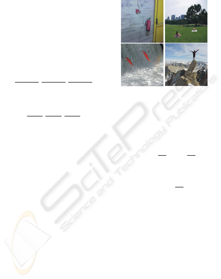
Figure 1 shows four input images which will be
used below, called extinguisher, park, fish and moun-
tain, all of size 256 × 256 pixels with 8 bits for
each colour component R, G and B. Figure 2 shows
three results of colour correction applied to the ex-
tinguisher image, from top-left to top-right: original
image, modified image with a blue tint (R –12%, G
+4% and B +50%), and modified image with a warm
white balance. The three results are shown below
the input images. As can be seen, colour correction
yields very similar images despite the rather large dif-
ferences in the input images. Colour correction as
explained above simulates colour constancy as em-
ployed in our visual system (Hubel, 1995).
Figure 1: Input images, left to right and top to bottom: ex-
tinguisher, park, fish and mountain.
The second step (b) is to reduce colour inhomo-
geneities in the images by adaptive smoothing of the
colour regions, while maintaining or even improving
the boundariesbetween different regions. We propose
a new, nonlinear, adaptive 1D filter, here explained in
the horizontal direction but it can be rotated, which
consists of a centred DOG
F
1,2
(x) = N
1

exp

−x
2
2σ
2
1

− exp

−x
2
2σ
2
2

, (3)
which is split into F
1
(x < 0) and F
2
(x > 0), and an-
other centred Gaussian, which is not split,
F
3
(x) = N
2
· exp

−x
2
2σ
2
2

, (4)
taking σ
1
≫ σ
2
. N
1
and N
2
are normalisation con-
stants which make the integrals of all three functions
equal to one. The three functions can be seen as a
simulation of a group of three cells at the same po-
sition, but with different dendritic fields which are
indirectly connected to cone receptors in the colour-
opponent channels a and b of Lab, F
3
yielding the
excitatory response of a receptive field of an on-
centre cell, and F
1,2
yielding excitatory responses of
two off-centre cells. From the three cell responses
R
1,2,3
we first compute the contrast between the left
(R
1
) and right (R
2
) responses; mathematically C =
|(R
1
− R
2
)/(R
1
+ R
2
)|. Then, based on the contrast
C and the minimum difference between the centre re-
sponse (R
3
) and the left and right responses, the out-
put R is determined by
R =

CR
1
+ (1−C)R
3
if |R
1
− R
3
| < |R
2
− R
3
|
CR
2
+ (1−C)R
3
otherwise.
(5)
VISAPP 2009 - International Conference on Computer Vision Theory and Applications
268

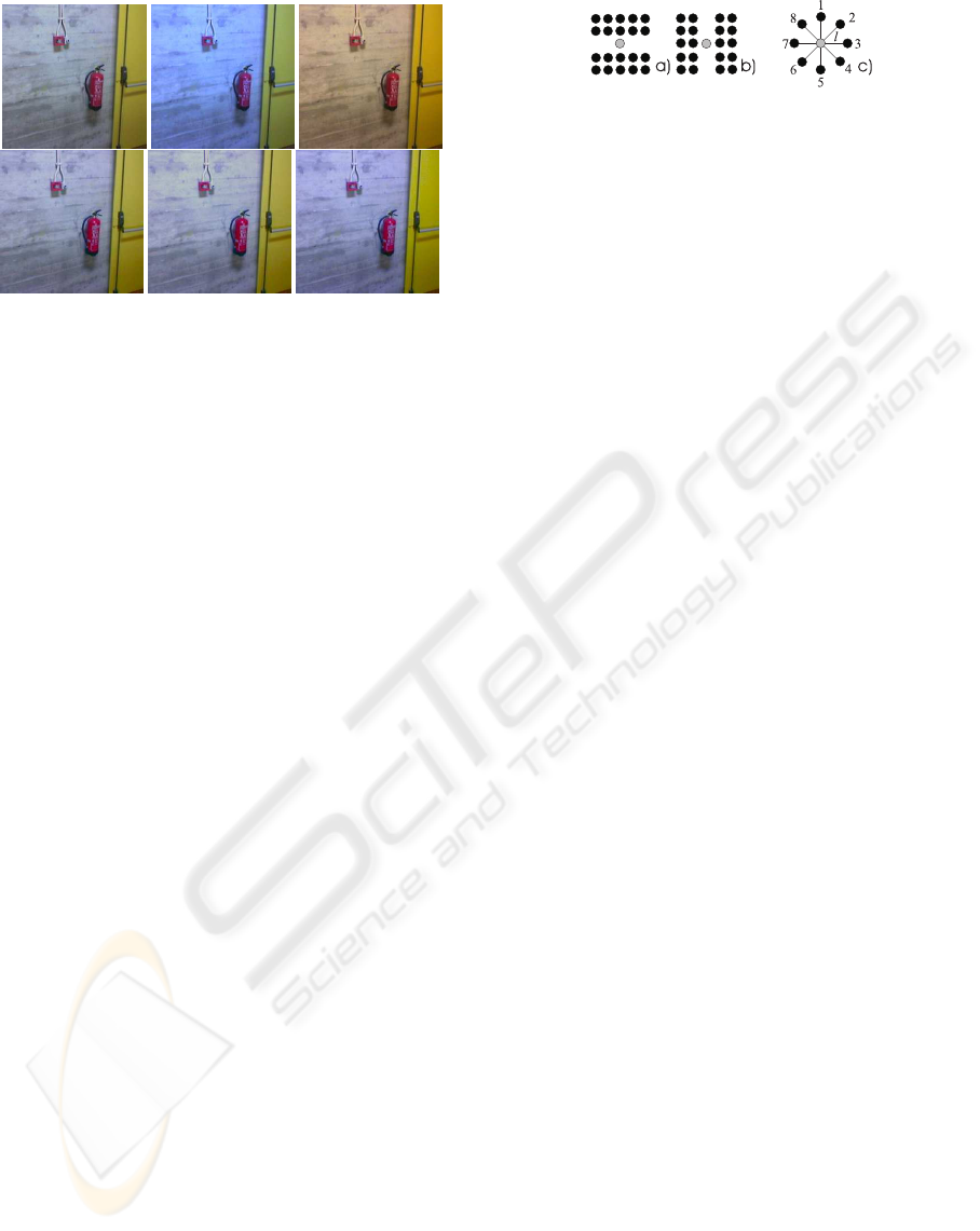
Figure 2: Colour illuminant and geometry normalisation.
Top: input images; bottom: respective results; see text.
In words, if the contrast is low, as in an almost ho-
mogeneous region, the filter support is big, but if the
contrast is high, at the boundary between two regions,
the filter support is small. This adaptive filtering is
applied to I
cc
at each pixel position (x,y), first hori-
zontally (R
H
) and then vertically (R
V
):
I
ci
(x,y) = R
V
[R
H
[I
cc
(x,y)]], (6)
where subscript ci stands for colour-improved. In our
experiments we obtained good results with σ
1
= 7 and
σ
2
= 3), and adaptive filtering in horizontal and verti-
cal directions was sufficient to sharpen blurred bound-
aries even with oblique orientations. Furthermore, the
processing is very fast because the three filter func-
tions need only be computed once.
After colour correction and adaptive filtering, the
third step (c) serves to detect boundaries. In fact,
for this purpose we could use the contrast function
C described above, but in order to accelerate process-
ing we apply a simple gradient operator, as shown in
Fig. 3a and b, which requires only two convolutions,
with mask sizes of 5× 2 and 2×5, of the components
of I
ci
. These masks can be seen as dendritic fields of
two cells, the two results being subtracted by a third
cell which combines horizontal and vertical gradients:
b
I
ed
(x,y) =
∑
left
I
ci
(x,y) −
∑
right
I
ci
(x,y)
+
∑
top
I
ci
(x,y) −
∑
bottom
I
ci
(x,y).
(7)
b
I
ed
(x,y) is then thresholded using
I
ed
(x,y) =

1 if
b
I
ed
(x,y) > k
0 otherwise,
(8)
where subscript ed stands for edge-detected. This
yields a binary edge map by means of a cell layer
in which cells are either active (response 1) or in-
active (response 0). We apply a global threshold
Figure 3: Gradient operators in vertical (a) and horizontal
(b) orientations with summation areas of 2 × 5 pixels, and
(c) the cluster of gating cells used for colour conspicuity.
k = max(I
ci
(x,y)). Edge detection yields three dis-
tinct maps, one for each component of Lab colour
space, I
L
ed
, I
a
ed
and I
b
ed
, which can be combined.
In the last step (d), colour conspicuity at colour
edges is calculated at each position in the edge map
where there is an active cell (I
L,a,b
ed
(x,y) = 1). We
define conspicuity Ψ at position (x,y) as the max-
imum difference between the colours in I
ci
at four
pairs of symmetric points at distance l from (x, y),
i.e., on horizontal, vertical and two diagonal lines.
Figure 3c shows a cluster of gating cells. If the gat-
ing cells are called G
i
, opposing pairs are (G
i
,G
i+4
),
with i = {1,...,4}, for example (G
1
,G
5
). Partial con-
spicuity is then calculated independently for each of
the colour components in Lab space, as defined by
(9a), where ~x
i
denotes the position of G
i
relative to
position (x, y). The final value is then calculated us-
ing the sum of all three colour components (9b).
Ψ
L,a,b
(x,y) = max
i

|I
L,a,b
ci
(~x
i
) − I
L,a,b
ci
(~x
i+4
)|

, (9a)
Ψ
Lab
(x,y) = Ψ
L
(x,y) + Ψ
a
(x,y) + Ψ
b
(x,y). (9b)
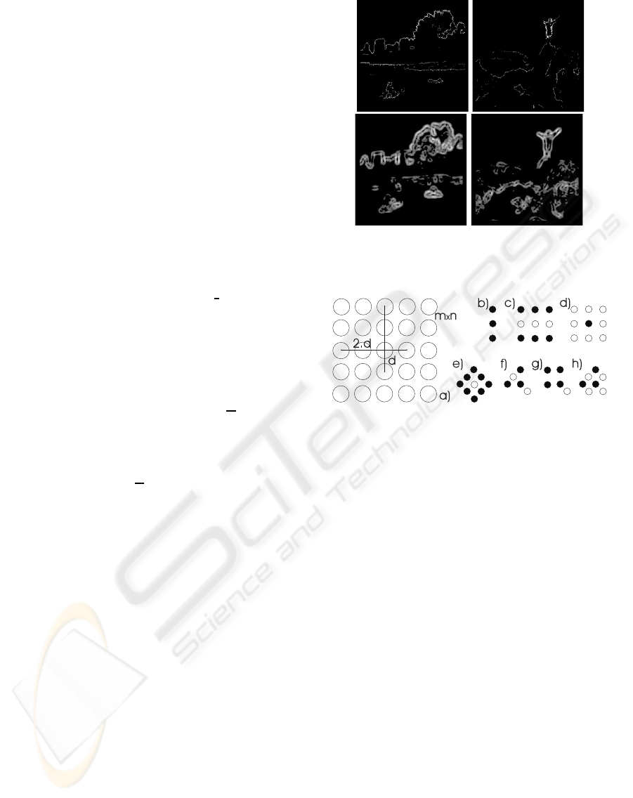
Results of colour conspicuity are shown in Fig. 4 top,
for the park and mountain images, using l = 4.
3 TEXTURE BOUNDARIES
Colour conspicuity Ψ
Lab
includes the luminance com-
ponent L and therefore luminance gradients, both in
coloured image regions and in non-coloured or gray
ones, but the processing as applied up to here is too
local to capture texture as a region property. As dif-
ferent colours in surrounding or neighbouring regions
attract attention, so do different textures because tex-
ture conveys complexity and therefore importance of
regions to attend for screening.
Texture processing is in principle completely
equal to colour processing, with adaptive filtering,
gradient detection and the attribution of conspicuity
to texture boundaries, but instead of using the three
Lab components only the L one is used and texture
features must be extracted from L(x,y). Since we are
developing biologically plausible methods, it makes
sense to apply Gabor wavelets as a model of corti-
cal simple cells. Although very sophisticated texture
FOCUS OF ATTENTION AND REGION SEGREGATION BY LOW-LEVEL GEOMETRY
269

models have been proposed on the basis of the Ga-
bor model (du Buf, 2007), we will only use the spec-
tral decomposition here because of speed. This frees
CPU time for applying a reasonable number of fre-
quency (scale) and orientation channels, which will
be 8× 8 = 64 in this paper. Since Gabor filtering in-
volves filter kernels which are relatively small (high-
frequency textures because of viewing distance), all
filtering can be done in the frequency domain (see e.g.
Rodrigues and du Buf (2004)) and requires one for-
ward FFT and 64 inverse FFTs, the latter parallelised
on multi-core CPUs or even graphics boards (GPUs).
In the spatial domain, Gabor filters consist of a
real cosine and an imaginary sine component, both
with a Gaussian envelope, which resemble receptive
fields of simple cells with even R
E
s,i
and odd symmetry
R
O
s,i
, with i the orientation and s the scale. Responses
of complex cells are modelled by taking the modulus
C
s,i
(x,y) = [{R
E
s,i
(x,y)}
2
+ {R
O
s,i
(x,y)}
2
]
1
2
.
Texture boundaries are obtained by applying three
processing steps to the responses of complex cells,
at each individual scale and orientation, after which
results are combined: (a) the responses C
s,i
(x,y) are
smoothed using the adaptive filter defined by eqns (3)
to (5), obtaining
b
C
s,i
. The next step (b) consists of
horizontal and vertical gradient detection C
s,i
, apply-
ing cells with dendritic fields of size 2× 5 as shown
in Fig. 3a, b to C
s,i
(x,y). The final step (c) consists of
summing the results at all scales and orientations
R(x,y) =
∑
s,i
C
s,i
(x,y), (10)
together with an inhibition of all responses below a
threshold (we apply 0.1max{R(x,y)}). Figure 4 (bot-
tom) shows the results in the case of park and moun-
tain. As can be seen, the information is more diffuse
and complements that of colour processing (top).
4 SALIENCY MAP
A saliency map is built on top of colour conspicuity
and texture boundary maps by using grouping cells
which code local geometry. There are two levels of
grouping cells. At the first, lower level, there are sum-
mation cells with a dendritic field size of n × m, with
the centres at a distance d; see Fig. 5a. In this paper
we use m = n = 5 and d = 5, such that the dendritic
fields of the cells do not overlap. These cells sum ac-
tivities in the colour or texture maps, hence boundary
conspicuity at individual pixel positions is reinforced
at this level, but also at the next level which deals with
local geometry. At the second level, there are many
grouping cells, each one devoted to one geometric
Figure 4: Colour boundary conspicuity (top) for images
park (left) and mountain (right). Bottom: texture bound-
aries.
Figure 5: Grouping cells for low-level geometry: (a) cluster
of cells with their dendritic fields (circles) on a 5 × 5 grid;
(b) to (h) show examples of spatial configurations.
configuration on a 5× 5 grid, but not all axons of the
cells at the lower level are used. This allows a sim-
ple construction of spatial configurations, as shown in
Fig. 5b to h, with up to four rotations, i.e., horizontal,
vertical and two diagonal orientations. The solid and
open circles in Fig. 5b to h refer to the use of the re-
sponses of the underlying summation cells: in case of
a solid circle the sum S needs to be positive (S > 0),
in case of an open circle S = 0, and responses of all
other summation cells on the grid are not used (they
are “don’t care”). Cells at this level take the maximum
of the responses of the excitated grouping cells, but
only if the spatial configuration of the non-excitated
grouping cells is correct. If the response R of con-
figuration c is R
c
, and if we call the configuration of
cells which must be excitated Ω
c
e
and that of the cells
which must not be excitated Ω
c
ne
, with Ω
c
e
,Ω
c
ne
∈ Ω,
the 5× 5 grid, and Ω
c
e
∧ Ω
c
ne
= 0, then
R
c
= max
i∈Ω
c
e
S
i
⇐
∑
j∈Ω
c
ne
S
j
= 0. (11)
The configurations shown in Fig. 5b to h concern, re-
spectively, a line (or an isolated contour), a bar (two
parallel contours of a bar), two types of blobs and
three types of corners. The d and e configurations are
VISAPP 2009 - International Conference on Computer Vision Theory and Applications
270

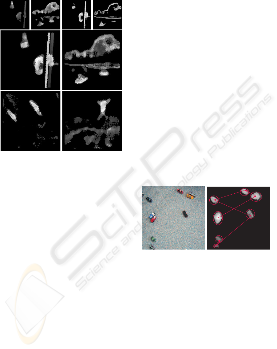
Figure 6: Saliency maps obtained by using only texture
boundaries (top-left), only colour conspicuity (top-right),
and by combining colour and texture (big images).
not rotated, but the other five are (horizontal, vertical
and two diagonal orientations), so in total there are 22
configurations c in the total set C. Since there may
be more configurations valid at the same position, the
last cell layer determines the response of the maxi-
mum configuration, which yields the saliency map:
R(x,y) = max
c∈C
R
c
(x,y). (12)
The top row of Fig. 6 shows results obtained when
using only texture boundaries(at left), and those when
using only colour conspicuity (at right). As can be
seen, the maps are different but they complement each
other, i.e., texture in general yields more diffuse ar-
eas (park and mountain images) whereas colour con-
spicuity is more concentrated on contours. Combined
results, using texture and colour, of all four images
are shown in the lower part of Fig. 6. These final
maps were created by taking the sum of the two val-
ues of the texture and colour saliency maps at each
pixel position. It should be stressed that all images
were normalised for visualisation purpose, darker ar-
eas corresponding to less saliency and brighter ones
to more saliency.
5 DISCUSSION
We introduced a simple, new, and biologically plau-
sible model for obtaining saliency maps based on
colour conspicuity and texture boundaries. The model
yields very good results in the case of natural scenes.
In contrast to the methods employed by Itti and Koch
(2001), whose saliency maps are very diffuse versions
of entire input images, our method is able to highlight
regions, a sort of pre-segregation of complex and con-
spicuous regions which is later required for precise
object segregation in combination with object cate-
gorisation and recognition.
The saliency maps provide crucial information
for sequential screening of image regions for object
recognition and tracking: FoA by fixating conspicu-
ous regions, from the most important regions to the
least important ones. Figure 7 shows an input im-
age with toy cars (left), the saliency map (right), and
the order, indicated by arrows, in which the regions
will be processed. Fixation points were selected auto-
matically by determining the highest response in the
saliency map within each region, and regions are fix-
ated using inhibition-of-return. Despite the fact that
saliency based on texture boundaries is more diffuse
than that on the basis of colour conspicuity, car-region
segregation is rather precise. The main reason for
this precision is that low-level geometry processing
mainly occurs at contours and inside objects, i.e., it
does not lead to region growing.
Figure 7: Toy cars image (left) and FoA-driven sequential
screening of regions (right).
The saliency model is now being extended by mo-
tion and disparity information, after which it can be
integrated into a complete architecture for invariant
object categorization and recognition (Rodrigues and
du Buf, 2006, 2007), which is based on multi-scale
keypoints, lines and edges derived from responses of
cortical simple, complex and end-stopped cells. This
is beyond the scope of this paper, but, as mentioned
in the Introduction, very fast global and local gist vi-
sion are two basic building blocks of an integrated
system. Until here, low-level geometry processing
has only been used for producing saliency maps for
FoA with segregated regions. But since low-level ge-
ometry information has already been extracted, it is
therefore available for obtaining local object gist, for
example providing cues which are used for a first and
FOCUS OF ATTENTION AND REGION SEGREGATION BY LOW-LEVEL GEOMETRY
271

fast selection of possible object categories in memory
(Bar M., et al., 2006). This is a purely bottom-up and
data-parallel process for bootstrapping the serial ob-
ject categorization and recognition processes which
are controlled by top-down attention. Low-level ge-
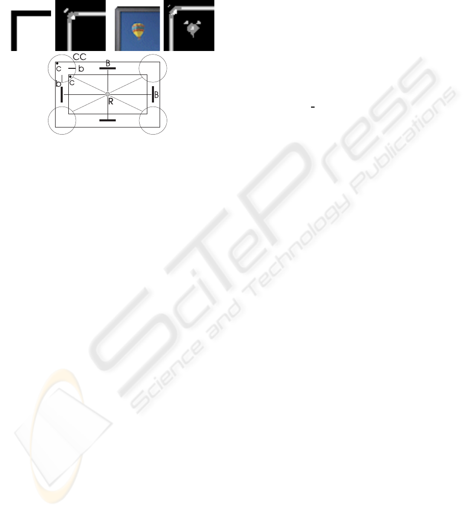
Figure 8: Low-level geometry (top) and example of mid-
and high-level geometry groupings (bottom); see text for
details.
ometry is difficult to visualise, because it consists of a
large number of spatial maps, in this paper limited to
22 but there could be more, one for each spatial con-
figuration. Figure 8 (top), shows detail images with a
few configurations coded by different levels of gray,
i.e., corners, bars and blobs. The input was an ideal
rectangle with two sharp corners (left) and a com-
puter monitor with a sharp inner corner but rounded
outer one. Despite the outer corner being rounded,
evidence for a corner has been detected at two pixel
positions. These results were obtained on the basis of
colour conspicuity, but later texture and colour infor-
mation should be combined, and low-level geometry
should be used to construct mid- and high-levelgeom-
etry. The latter idea is illustrated in Fig. 8 (bottom):
at low level corners (c) and bars (b) are detected. At
mid level, these can be grouped into a complex corner
(CC), and at high level the CCs, together with linking
bars B, into a rectangle R. Such an R structure is typ-
ical for man-made objects, for example a computer
monitor or a photo frame. This example of high-level
geometry is perhaps the last level below semantic pro-
cessing: a computer monitor in combination with one
or more photo frames is an indication for global scene
gist: our office. In any case, the large number of fea-
tures at the lowest level (64 Gabor channels) is re-
duced to the number of spatial configurations at low-
level geometry, here 22. Groupings at mid level (e.g.,
complex corner CC) may lead to less configurations,
but at high level (e.g., rectangle R) the number of con-
figurations will increase again, because many elemen-
tary shapes must be represented. On the other hand,
the precise localisation of configurations which is re-
quired at low level is not necessary at higher levels;
for example, grouping cells for complex corners CC
may be located somewhere near the centres of the cir-
cles in Fig. 8 (bottom), as long as their dendritic fields
are big enough to receive input from two corner and
two bar cells. These aspects are subject to further re-
search.
ACKNOWLEDGEMENTS
Research supported by the Portuguese Foundation for
Science and Technology (FCT), through the pluri-
annual funding of the Inst. for Systems and Robotics
through the POS Conhecimento Program (includes
FEDER funds), and by the FCT project SmartVision:
active vision for the blind (PTDC/EIA/73633/2006).
REFERENCES
Bar M., et al. (2006). Top-down facilitation of visual recog-
nition. PNAS, 103(2):449–454.
du Buf, J. (2007). Improved grating and bar cell models in
cortical area V1 and texture coding. Image and Vision
Computing, 25(6):873–882.
Elazary, L. and Itti, L. (2008). Interesting objects are visu-
ally salient. Journal of Vision, 8(3):1–15.
Finlayson, G., Schiele, B., and Crowley, J. (1998). Compre-
hensive colour image normalization. Proc. 5th Europ.
Conf. Comp. Vision, I:475–490.
Hubel, D. (1995). Eye, brain and vision. Scientific Ameri-
can Library.
Itti, L. and Koch, C. (2001). Computational modeling
of visual attention. Nature Reviews: Neuroscience,
2(3):194–203.
Niebur, E. and Koch, C. (1996). Control of selective vi-
sual attention: Modeling the ‘where’ pathway. Neural
Information Processing Systems, 8:802–808.
Rensink, R. (2000). The dynamic representation of scenes.
Visual Cogn., 7(1-3):17–42.
Rodrigues, J. and du Buf, J. (2004). Visual cortex fron-
tend: integrating lines, edges, keypoints and disparity.
Proc. Int. Conf. Image Anal. Recogn., Springer LNCS
3211(1):664–671.
Rodrigues, J. and du Buf, J. (2006). Multi-scale keypoints
in V1 and beyond: object segregation, scale selection,
saliency maps and face detection. BioSystems, 2:75–
90.
Rodrigues, J. and du Buf, J. (2007). Invariant multi-
scale object categorisation and recognition. Proc.
3rd Iberian Conf. on Patt. Recogn. and Image Anal.,
Springer LNCS 4477:459–466.
van de Weijer, J., Gevers, T., and Bagdanov, A. D. (2006).
Boosting color saliency in image feature detection.
IEEE Tr. PAMI, 28(1):150–156.
VISAPP 2009 - International Conference on Computer Vision Theory and Applications
272