IMPROVING CLASSIFICATION FOR BRAIN COMPUTER

INTERFACES USING TRANSITIONS AND A MOVING WINDOW

Ricardo Aler, In´es M. Galv´an and Jos´e M. Valls

Computer Science Department, Universidad Carlos III de Madrid, Avda. Universidad, 30, Legan´es, Spain

Keywords:

Brain Computer Interface, Machine learning.

Abstract:

The context of this paper is the brain-computer interface (BCI), and in particular the classiﬁcation of signals

with machine learning methods. In this paper we intend to improve classiﬁcation accuracy by taking advantage

of a feature of BCIs: instances run in sequences belonging to the same class. In that case, the classiﬁcation

problem can be reformulated into two subproblems: detecting class transitions and determining the class for

sequences of instances between transitions. We detect a transition when the Euclidean distance between the

power spectra at two different times is larger than a threshold. To tackle the second problem, instances are

classiﬁed by taking into account, not just the prediction for that instance, but a moving window of predictions

for previous instances. Our results are competitive with those obtained in the BCI III competition.

1 INTRODUCTION

The context of this paper is the brain-computer in-

terface (BCI), a growing research ﬁeld, that would

allow users to control computers and other devices

by means of brain signals (Curran and Stokes, 2003),

(Millan J del R and Gerstner, 2004) (G. Pfurtscheller

and Birbaumer, 2005), (Kubler and Muller, 2007).

One of the main problems of BCI is to accurately

decode individual brain signals. Machine Learning

techniques are typically applied here, by training clas-

siﬁers with the brain signals of the user that is going

to use the interface (Dornhege et al., 2007). For in-

stance, a BCI can be trained to recognize three dif-

ferent classes corresponding to three different mental

states: left-hand motor imagery, right-hand motor im-

agery, and object rotation imagery.

Noisy weak signals and high variability between

same-user sessions

make the classiﬁcation problem

difﬁcult, resulting in many on-line classiﬁcation er-

rors, frustated users, and low transfer (speed) rates

from the user to the computer. The transfer rate could

be increased if three or more classes are used. How-

ever, multi-class classiﬁcation problems are more dif-

ﬁcult than two-class ones.

This means that the classiﬁer learned during one ses-

sion might not be accurate in the next session, even for the

same user.

In this paper we intend to improve classiﬁcation

accuracy by taking advantageof a feature of BCIs: in-

stances run in sequences belonging to the same class

(for instance, right-hand motor imagery), followed by

a transition into a different class. Typically, the BCI

classiﬁcation problem is tackled by trying to classify

the EEG signal at every instant in time. However,

given that classes run in sequences, the classiﬁcation

problem can be reformulated into two subproblems:

• Detecting class transitions

• Determining the class for sequences of instances

between transitions.

The ﬁrst problem can be approached in many dif-

ferent ways. In this paper we detect transitions by

computing the Euclidean distance between the power

spectra at two different times (samples) and signalling

a class transition when the distance is larger than a

threshold.

By detecting transitions, the accuracy of the sec-

ond problem (classiﬁcation between transitions) can

also be improved in two ways. First, if the class of

the last sequence (before the transition) is known, that

class can be discarded after the transition, hence be-

coming a simpler N-1 class classiﬁcation problem.

Also, sequences may contain many instances (de-

pending of the sampling rate), but only a few are nec-

essary to determine the class of the whole sequence.

This is actually no different than determining if a coin

Aler R., Galván I. and Valls J. (2009).

IMPROVING CLASSIFICATION FOR BRAIN COMPUTER INTERFACES USING TRANSITIONS AND A MOVING WINDOW.

In Proceedings of the International Conference on Bio-inspired Systems and Signal Processing, pages 65-71

DOI: 10.5220/0001535800650071

 SciTePress

is biased towards heads or tails, based on a small sam-

ple of coin tosses. We use a similar idea in this paper.

We have applied these ideas to the data supplied for

the BCI III competition. The datasets are described

in Section 2. The method is described in Section 3.

Section 4 shows the obtained results. Section 5 sum-

marizes our results and draws some conclusions.

2 DESCRIPTION OF EEG DATA

In this paper we are going to use a high quality dataset

acquired in the IDIAP Research Institute by Silvia

Chiappa and Jos del R. Milln (Mill´an, 2004). It was

used in the BCI-III competition that took place in

2005.

This dataset contains data from 3 normal sub-

jects during 4 non-feedback sessions. The subjects sat

in a normal chair, relaxed arms resting on their legs.

There are 3 tasks, so this is a three-class classiﬁcation

problem:

• Imagination of repetitive self-paced left hand

movements

• Imagination of repetitive self-paced right hand

movements

• Generation of words beginning with the same ran-

dom letter

All 4 sessions of a given subject were acquired

on the same day, each lasting 4 minutes with 5-10

minutes breaks in between them. The subject per-

formed a given task for about 15 seconds and then

switched randomly to another task at the operator’s

request. EEG data is not splitted in trials since the

subjects are continuously performing any of the men-

tal tasks. Data was provided in two ways: raw EEG

signals, and data with precomputed features. In this

paper, we use the precomputed dataset.

Features were precomputed as follows. The raw

EEG potentials were ﬁrst spatially ﬁltered by means

of a surface Laplacian. Then, every 62.5 ms (i.e., 16

times per second) the power spectral density (PSD)

in the band 8-30 Hz was estimated over the last sec-

ond of data with a frequency resolution of 2 Hz for

the 8 centro-parietal channels C3, Cz, C4, CP1, CP2,

P3, Pz, and P4. As a result, an EEG sample is a 96-

dimensional vector (8 channels times 12 frequency

components).

In summary, in this paper we are going to tackle

a three-class classiﬁcation problem with 96 input at-

tributes, which deﬁne the PSD over 62.5 ms for 8

input channels. There are three subjects, with four

http : //ida. first. fraunhofer.de/projects

/bci/competition iii/.

datasets (sessions) for each one: three datasets for

training and one dataset for testing.

3 METHOD

The method used here to improve BCI classiﬁcation

accuracy based on assigning a class to a complete se-

quence of instances is based on two main ideas. First,

the transition in the signal from a class to another

class must be detected. This knowledge is used to

discard the class assigned to the previous sequence

of instances, just before the transition. Hence, the

prediction problem of N classes is transformed into a

prediction problem of N − 1 classes. Usually, in clas-

siﬁcation tasks the reduction of the number of classes

helps to increase the performance of the classiﬁcation

algorithm.

On the other hand, the proposed method is in-

spired in the idea that in this problem, the class

to predict remains ﬁxed for a time period that we

havecalled sequence of instances between transitions.

That means that, within a sequence, the class is not

continuously changing. Hence, it makes sense to try

to guess the class assigned to that sequence instead

of using the classiﬁer to predict each instance of the

sequence independently of each other. The simplest

way to assign a class to a sequence is to compute the

majority class returned by the classiﬁer on a small set

of instances at the beginning of the sequence. How-

ever, if the classiﬁer makes many mistakes at the be-

ginning of the sequence, the whole sequence will be

missclassiﬁed. In our ﬁrst approach, we tried to as-

sign a class to whole sequences based only on the ﬁrst

instances, and very frequently, complete sequences

were missclassiﬁed, and the whole method crashed.

Therefore, we have decided to classify the i

′

th in-

stance in the sequence by considering a moving win-

dow of the n previous instances. This gives some in-

ertia to the classiﬁer (it considers n instances instead

of just one), but if mistakes are made by the user,

the classiﬁer will recover eventually, once the mov-

ing window has gone past the mistaken instances. We

offer a well-founded method for selecting the window

size n, that it is explained at the end of the section.

Next, a detailed description of the method is pre-

sented. It includes the following parts: the procedure

to detect the transition; the procedure to select the

classiﬁer once the transition is detected and one of

the class is discarded; the procedure to classify test

instances with a moving window; and the mechanism

to compute the window size.

As we described in Section 2, we assume that the

original data in the time domain has been transformed

BIOSIGNALS 2009 - International Conference on Bio-inspired Systems and Signal Processing

to Power Spectral Density (PSD) in the frequency do-

main. Thus, we assume that we have a set of samples

(or instances) and every sample contains all the com-

ponents of the PSD for all channels at every instant.

That is:

sample



PSD

r, j

(i) j = 1,...,NoC, r = 1,...R



(1)

where PSD

r, j

(i) is the value of the r

spectral com-

ponent for the the j

channel, NoC is the number

of channels, and R is the number of components in

the PSD. For instance, if the PSD ranges from 8Hz

to 30Hz and there is a component every 2Hz (a 2Hz

resolution), R = 12.

Next, we describe the components of our method:

• Transition Detection. It is based on the observa-

tion that when a change of class occurs, a change

in the frequency domain also occurs. The idea

is to detect that transition by computing the Eu-

clidean distance between PSDs at two consecu-

tive samples. For every sample i, the distance

= ||PSD(i) − PSD(i− 1)|| between the PSD of

sample

and sample

i−1

is calculated as:

Noc

∑

j=1



∑

r=1

|PSD

r, j

(i) − PSD

r, j

(i− 1)|



(2)

Once the distance d

is obtained, a threshold value

U has to be set, such that if the distance is higher

that this threshold, a transition is signaled. The

value of U is crucial for successfully predict tran-

sitions and therefore, very important for the suc-

cess of the method.

In order to determine that threshold, the follow-

ing mechanism is applied. The training data set

X is divided into two subsets, named X

notransition

and X

transition

. The ﬁrst one, X

notransition

, con-

tains the samples for which there is no tran-

sition; and, the second one X

transition

contains

the transition samples. This separation can be

made because samples are labeled in the train-

ing set (i.e. their class is known), and there-

fore a transition is just a change of class. After

that, the distances d

for samples in X

notransition

are calculated and the maximum of these dis-

tances, named MaxDis

notransition

, is also obtained

. The distances d

for samples in subset X

transition

are also obtained and ranked from low to high.

Obviously, a good threshold U must be larger

than MaxDis

notransition

. We currently deﬁne U

as the next d

of set X

transition

that is larger than

MaxDis

notransition

. This way of setting the thresh-

old does not guarantee that all transitions will be

detected. However, this method is simple and rea-

sonable and later we will show that it performs

correctly on the test data.

• Choosing the Appropriate Classiﬁer, once the

Transition has been Detected. Let us remem-

ber that when a transition is detected, the class

of the previous sequence of instances is discarded

(i.e. after the transition, the class must change).

Therefore, after the transition, the system only

needs a classiﬁer that is able to classify sam-

ples (or instances) into N − 1 classes (discarding

the previous class). As the system must be pre-

pared for all classes, all (N − 1)-class classiﬁers

must be trained off-line using the training data,

prior to the system going on-line. If there are

N classes (C

to C

), there will be N (N − 1)-

class classiﬁers. The ﬁrst classiﬁer, named K

2,...,N

assumes that class C

is discarded and will pre-

dict the class in the set {C

,...,C

}. The sec-

ond classiﬁer, named K

1,3,...,N

, will discard class

and classify instances in N − 1 classes in the

set {C

,... ,C

}. The k

′

th classiﬁer, named

1,...k−1,k−1,...,N

, will consider only classes in the

set {C

,... ,C

k−1

k+1

,...,C

}. And so on, until

,...,C

N−1

}. Also, an N-class classiﬁer must be

learned, because at the beginning there is no pre-

vious sequence of samples, and therefore, no class

can be discarded. In this work, we have used Sup-

port Vector Machines (SVM) because they obtain

a very good performance(Vapnik,1998), although

any other machine learning algorithm could have

been employed.

The method is applied to predict the class in real

time (on-line). The main idea is to use one of

the classiﬁers for N − 1 classes, when a transition

is detected, instead of using the general classiﬁer

(the classiﬁer for N classes). Usually, the perfor-

mance of classiﬁers with fewer classes is higher

because if a class is removed, uncertainty about

the class is also reduced.

The procedure to select the classiﬁer in real-time

is described next: when the prediction process be-

gins, the N-class classiﬁer is responsible for pre-

diction. At the same time, the distances d

given

by equation 2 are calculated. When a transition

occurs (i.e. d

> U), one of the N classiﬁers for

N − 1 classes must be chosen. To choose the

most appropriate classiﬁer, the majority class pre-

dicted in the previous sequence of instances (i.e.,

the set of instances between the last two transi-

tions) must be discarded. Let’s suppose that the

In fact, we use Weka’s SMO implementation with stan-

dard parameters (a linear kernel and C = 1(Garner, 1995).

IMPROVING CLASSIFICATION FOR BRAIN COMPUTER INTERFACES USING TRANSITIONS AND A MOVING

WINDOW

class of the last sequence was k. Therefore, class

k will be ruled out for the current transition, and

the K

1,...k−1,k−1,...,N

classiﬁer will be responsible

for prediction during the current sequence until

the next transition is detected.

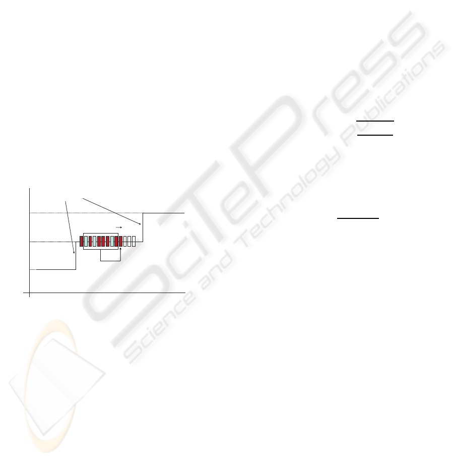
• Procedure to Classify Test Instances with a

Moving Window

As explained at the beginning of the section, we

use a second idea here to improve classiﬁcation

accuracy: in order to classify sample

, a window

with the predictions of the selected classiﬁer for

the n previous samples will be used, instead of

just using the prediction for sample

. This is sim-

ilar to determining if a biased coin is biased to-

wards heads based only on the n previousfew coin

tosses. Sample

will be classiﬁed as the major-

ity class of instances within the window. It is a

moving window because only the last n predic-

tions just before sample

are taken into account.

As the windows moves, all the samples inside it

are classiﬁed by the selected classiﬁer. Figure 1

shows how it works. The only remaining issue is

to estimate a ”good” window size n. This will be

done next.

Transitions

Class

Time

Movingwindow

Predictedinstance

Classa

Classb

Classc

......

ClassifierK

abc

Figure 1: Moving window to classify test instances.

• Computing the Size of the Moving Window

Assigning the majority class of instances within

the window to the next sample is reasonable, but

mistakes would occur if the frequencyof that class

in the window is not too far from 50%. This can

be solved by establishing a safe conﬁdence in-

terval around the estimated frequency. For sim-

pliﬁcation purposes, let’s suppose there are only

three classes (N = 3, classes a, b, and c), and as

explained before, one of them will be discarded

after the transition and one of the 3 2-class clas-

siﬁers will be used for the current sequence un-

til the next transition. Let’s suppose that class a

is discarded and therefore classiﬁer K

must be

used for the current sequence (K

separates class

b from class c). Although, the class of the current

sequence is ﬁxed until the next transition, the pre-

dictions of K

will make mistakes. In fact, just

like coin tosses, classiﬁcation errors follow a Bi-

nomial distribution (with success probability p).

If the actual class of the current sequence is b, the

distribution of mistakes of K

will follow a Bino-

mial distribution with p = TP

, where TP

the True Positive rate for class b and classiﬁer K

(i.e. the accuracy for class b obtained by classiﬁer

). On the other hand, if the actual class is c,

p = TP

If the actual class is b, p can be estimated ( ˆp) from

a limited set of instances (we call it ’the window’),

and from standard statistical theory (and by as-

suming the Binomial distribution can be approxi-

mated by a Gaussian), it is known that ˆp belongs

to a conﬁdence interval around p with conﬁdence

α:

ˆp ∈ p + −z

p(1− p)

(3)

where n is the size of the window. From Eq 3, we

can estimate the size of the window required:

n ≥ z

p(1− p)

(p− 0.5)

(4)

When generating predictions, the actual class of

the current sequence is not known, and there-

fore we have to assume the worst case, that

happens when p is closest to 0.5. There-

fore, p = min(TP

,TP

). To be in the

safe side, for this paper, we have decided

to make the window size independent of the

classiﬁer assigned to the current sequence.

Therefore, if there are three classes p =

min(TP

,TP

). A

similar analysis could be done for more than three

classes.

It is important to remark that Eq 4 is only a heuris-

tic approximation, since instances in a window are

not independent in the sense required by a Bi-

nomial distribution. For instance, if the user be-

comes tired and unfocused, s/he will generate a

sequence of noisy data that will be labeled uncor-

rectly. If the window includes that sequence of

mistakes, the classiﬁcation based on that window

will also be mistaken. However, the classiﬁer will

recover once the moving window goes past the se-

quence of mistakes.

BIOSIGNALS 2009 - International Conference on Bio-inspired Systems and Signal Processing

4 RESULTS

The aim of this Section is to show the results of our

method on the datasets described in Section 2. Let

us remember that there were three subjects, and each

one generated four sessions worth of data. The ﬁrst

three sessions are available for learning while session

four is only for testing. All datasets are three-class

classiﬁcation problems with classes named 2, 3, and

Our method computes all two-class SMO classi-

ﬁers. SMO is the Weka implementation of a Sup-

port Vector Machine. Table 1 displays the results of

all two-class classiﬁers (K

, K

) and the three-

class classiﬁer (K

237

). The training has been made

with sessions 1 and 2 instances and the testing with

session 3. The three-class classiﬁer accuracies can

be used as a baseline to compare further results. In

brackets we can observe the True Positive rate (TP)

for each class. For instance, 74.7 is the True Positive

rate (TP) for class 2 for the K

two-class classiﬁer

(i.e. TP

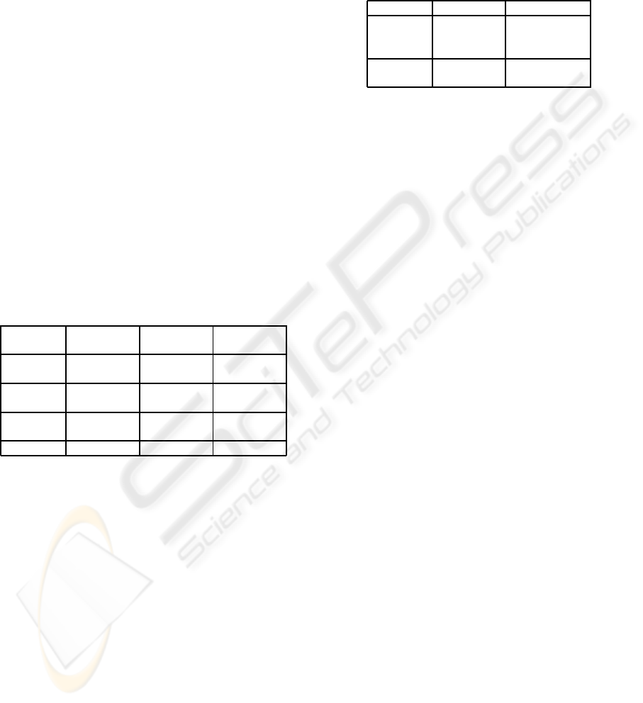
Table 1: Accuracy of two-class and three-class SMO clas-

siﬁers for subjects 1, 2, and 3. Training with sessions 1 and

2, and testing with session 3.

SMO Subject 1 Subject 2 Subject 3

Classiﬁer

79.0 71.9 52.3

(74.7/83.8) (68.2/75.3) (53.3/51.4)

82.4 74.3 57.9

(64.8/93.9) (62.7/81.9) (50.6/65.2)

83.0 76.8 60.4

(81.2/84.4) (63.5/87.7) (54.9/65.9)

237

73.8 62.0 40.9

Section 3 gives the details for computing the

thresholds for detecting transitions. These are: U

0.563108963, U

= 0.58576, U

= 0.587790606, for

subjects 1, 2, and 3, respectively.

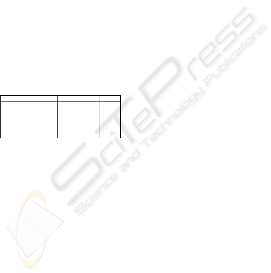
Our method uses the TP rate (class accuracy), ob-

tained with session 3, for computing the moving win-

dow size, according to Eq 4. p will be set as the

minimum of all TP rates. So we have p

= 0.648,

= 0.627, and p

= 0.506 for subjects 1, 2, and

3, respectively. A conﬁdence interval with α = 0.99

will be used, therefore z

= 2,5759. Table 2 displays

the windows sizes for every subject. It can be seen

that the window size for subject 3 requires 46072 in-

stances many more than available, so we apply the

window moving idea only to subjects 1 and 2. This

is due to the accuracy of classiﬁers for subject 3 are

very low, in particular the accuracy of K

(see Table

1). We have also computed the window size for larger

probabilities to check the performance of the method

if smaller window sizes are used. For instance, we

have also considered p

= 0.80 and p

= 0.70 (those

values are approximately the accuracies of the two-

class classiﬁers in Table 1).

Table 2: Window size used for subjects 1, 2, and 3.

Probability Window Size

Subject 1 0.648 78

Subject 2 0.627 92

Subject 3 0.506 46072

Subject 1 0.80 12

Subject 2 0.70 92

Finally, Table 3 shows the ﬁnal results. The ﬁrst

row displays the competition results (Galan et al.,

2005) on session four. (Galan et al., 2005) proposed

an algorithm based on canonical variates transforma-

tion and distance based discriminant analysis com-

bined with a mental tasks transitions detector. As re-

quired by the competition, the authors compute the

class from 1 second segments and therefore no win-

dows of samples are used. The second row, displays

the best results from the competition using longer

windows (Gan and Tsui, 2005) (it reduces dimension-

ality of data by means of PCA and the classiﬁcation

algorithm is based on Linear Discrimination Analy-

sis). No details are given for the size of the win-

dow of samples. The third row shows the results of

the three-class classiﬁer (sessions 1 and 2 were used

for training and session 4, for testing). The fourth

row contains the results (on session four) of apply-

ing the transition detector only. In this case, once the

transition is detected, the previous class is discarded

and the prediction is made using the two-class clas-

siﬁer chosen. These results are better than the three-

class classiﬁer. For subject 3, the performance of the

method using the transition detection is very low be-

cause some of the two-class classiﬁers for subject 3

have a very low accuracy (see K

in Table 1). Let us

remember that when a transition is detected, the pre-

vious class is discarded. The previous class is com-

puted as the majority class of the previous sequence.

If the classiﬁer used in the previous sequence is very

bad, the majority class might not be the actual class.

Hence, the wrong class would be discarded in the cur-

rent sequence, and the wrong 2-class classiﬁer would

be selected. That would generate more mistakes that

would be propagated into the next sequence, and so

on. Given that all samples between transitions are

used to compute the previous class and that the (N-

1) classiﬁers are better than chance, the possibility of

mistaking the previous class is very low. In fact, for

the data used in this article, this situation has not oc-

curred. But it is important to remark that preventing

the propagation of the missclassiﬁcation of the previ-

IMPROVING CLASSIFICATION FOR BRAIN COMPUTER INTERFACES USING TRANSITIONS AND A MOVING

WINDOW

ous class is crucial for the success of the method and

we intend to improve this aspect in the future.

The ﬁfth row in Table 3 shows the results with

the method described in Section 3. In this case, both

ideas, the transition detection and the moving win-

dow size, are used. Results improve signiﬁcantly if

the moving window is used: classiﬁcation accuracy

raises from 74.8 to 94.8 and from 74.6 to 86.3 (sub-

jects 1 and 2, respectively). It can also be seen that

results are also improved if a smaller window size is

used (MW with small sample).

Comparing our method with the best competition

result that used a window of samples (second row of

Table 3), we can see that our method is competitive

with respect to the ﬁrst subject and improves the per-

formance for the second subject. Unfortunately our

method cannot be applied to the third subject due to

the large number of samples required for the window.

It can also be seen that using windows improves accu-

racy signiﬁcatively (second, ﬁfth, and sixth rows ver-

sus the ﬁrst one of Table 3).

Table 3: Results for subjects 1, 2, and 3.

Subj. 1 Subj. 2 Subj. 3

BCI comp. (1 sec.) 79.60 70.31 56.02

BCI comp. (long window) 95.98 79.49 67.43

3-class classiﬁer 74.8 60.7 50.2

Transition detector 80.8 74.6 52.2

Moving window 94.8 86.3 -

MW small sample 84.2 82.5 -

5 SUMMARY AND

CONCLUSIONS

Typically, in BCI classiﬁcation problems EEG sam-

ples are classiﬁed at every instant in time indepen-

dently of previous samples. These samples run in

sequences belonging to the same class, and then fol-

lowed by a transition into a different class. We present

a method that takes this fact into consideration with

the aim of improving the classiﬁcation accuracy. The

general classiﬁcation problem is divided into two sub-

problems: detecting class transitions and determin-

ing the class between transitions. Class transitions

are detected by computing the Euclidean distance be-

tween PSD at two consecutive times; if the distance

is larger than a certain threshold then a class tran-

sition is detected. Threshold values are automati-

cally determined by the method. Once transitions

can be detected, the second subproblem -determining

the class between transitions- is considered. First,

since the class before the transition is known, it can

be discarded after the transition and therefore, a N-

class problem becomes a (N-1)-class problem, which

is easier. Second, sequences between two transitions

may contain many instances but only a few are nec-

essary to determine the class of the whole sequence.

In order to determine the class between transitions a

moving window is used to predict the class of each

testing instance in such a way that only the n last pre-

dictions before the testing instance are taken into ac-

count. The estimation of the window size (n) is based

on standard statistical theory.

This method has been applied to a high quality

dataset which had been previously precomputed, re-

sulting in a three-class classiﬁcation problem with 96

input attributes. These data corresponds to three sub-

jects, with four sessions for each one: three for train-

ing and one for testing. Several experiments have

been done in order to validate the method and the ob-

tained results show that just by applying the transition

detector, the classiﬁcation rates are better than when

a 3-class classiﬁer is used. When the moving window

is used, the results are signiﬁcatively better. Those

results are also competitive to those obtained in the

BCI competition: similar for subject 1, better for sub-

ject 2, and worse for subject 3. We also show that if

a smaller window size is used the classiﬁcation rates

are also better than those that use only the transition

detector and the three-class classiﬁer.

REFERENCES

Curran, E. and Stokes, M. (2003). Learning to control brain

activity: a review of the production and control of eeg

components for driving braincomputer interface (bci)

systems. Brain Cognition, 51.

Dornhege, G., Krauledat, M., Muller, K.-R., and Blankertz,

B. (2007). Toward Brain-Computer Interfacing, chap-

ter General Signal Processing and MAchine Learning

Tools for BCI Analysis, pages 207–234. MIT Press.

G. Pfurtscheller, C. N. and Birbaumer, N. (2005). Mo-

tor Cortex in Voluntary Movements, chapter 14, pages

367–401. CRC Press.

Galan, F., Oliva, F., and Guardia, J. (2005). Bci competi-

tion iii. data set v: Algorithm description. In Brain

Computer Interfaces Competition III.

Gan, J. Q. and Tsui, L. C. (2005). Bci competition iii. data

set v: Algorithm description. In Brain Computer In-

terfaces Competition III.

Garner, S. (1995). Weka: The waikato environment for

knowledge analysis. In S.R. Garner. WEKA: The

waikato environment for knowledge analysis. In Proc.

of the New Zealand Computer Science Research Stu-

dents Conference, pages 57–64.

BIOSIGNALS 2009 - International Conference on Bio-inspired Systems and Signal Processing

Kubler, A. and Muller, K.-R. (2007). Toward Brain-

Computer Interfacing, chapter An Introduction to

Brain-Computer Interfacing, pages 1–26. MIT Press.

Mill´an, J. (2004). On the need for on-line learning in

brain-computer interfaces. In Proceedings of the In-

ternational Joint Conference on Neural Networks, Bu-

dapest, Hungary. IDIAP-RR 03-30.

Millan J del R, Renkens F, M. J. and Gerstner, W. (2004).

Noninvasive brain-actuated control of a mobile robot

by human eeg. IEEE Trans Biomed Eng, 51.

Vapnik, V. (1998). Statistical Learning Theory. John Wiley

and Sons.

IMPROVING CLASSIFICATION FOR BRAIN COMPUTER INTERFACES USING TRANSITIONS AND A MOVING

WINDOW