
THERMOGRAPHIC BODY TEMPERATURE MEASUREMENT
USING A MEAN-SHIFT TRACKER
Guillaume-Alexandre Bilodeau
1
, Maxime Levesque
2
, J. M. Pierre Langlois
1
Pablo Lema
2
and Lionel Carmant
2
1
D´epartement de g´enie informatique et g´enie logiciel,
´
Ecole Polytechnique de Montr´eal
P.O. Box 6079, Station Centre-ville, Montr´eal (Qu´ebec), H3C 3A7, Canada
2
Pediatry, Sainte-Justine Hospital, 3175, Cˆote Ste-Catherine, Montr´eal (Qu´ebec), H3T 1C5, Canada
Keywords:
Thermography, Mean-Shift Tracker, Temperature measurement, Epilepsy.
Abstract:
In epilepsy research, using a wide range of sensors can help to automatically detect the occurrence of seizures
and to understand their underlying mechanisms. One such sensor is a thermographic camera that can measure
the surface temperature of the body. This sensor may have an important role in investigating seizures as
studies have shown that they can affect the body temperature of a patient. Furthermore, it has also been
shown that kainic acid, a drug used to provoke seizures in animals, has an impact on rat body temperature.
Consequently, there is a need to continuously measure the evolution of the body temperature of an animal
during seizures. In this paper, we present our developed methodology to measure the temperature of a moving
rat using a thermographic camera. To accurately measure the body temperature, we propose a methodology
using a Mean-Shift tracker. The obtained measures are compared with a ground truth. The method is tested
on a 2-hour video, and it is shown that the Mean-Shift tracker achieves an RMS error of approximately 0.1
◦
C.
1 INTRODUCTION
Neonatal seizures are convulsive events in the first
28 days of life in term infants or for premature in-
fants within 44 completed weeks of conceptional age.
Neonatal seizures are the most frequent major man-
ifestation of neonatal neurologic disorders (Volpe,
1989). Population-based studies of neonatal seizures
in North America report rates between 1 and 3.5 per
1000 live births. Most neonatal seizures begin early,
with almost half on the first day of life and two-thirds
within the first 2 days of life. During the neonatal
period, the brain is most susceptible to the occur-
rence of seizures because of an excess of excitatory
neurons and the inhibitory neurotransmitter GABA
plays an excitatory role. Initially thought to have lit-
tle long-term consequences, we have more and more
evidence that these seizures are deleterious to the de-
veloping brain (Carmant, 2006). Therefore, more
emphasis is put on the treatment of these early life
seizures. However, due to the immature connections
in the neonatal brain, these seizures exhibit unusual
clinical patterns, mimic normal movements and have
primitive EEG patterns that are not easily recogniz-
able. Therefore, one would be required to monitor all
at-risk newborns continuously to confirm the epilep-
tic nature of their events. At Ste-Justine Hospital,
in Montreal, Canada, this typically represents 40 pa-
tients at any one time. For this reason, several au-
thors have addressed automatic detection of neonatal
seizures using video recordings or electroencephalo-
gram (EEG) pattern recognition (Karayiannis et al.,
2001; Karayiannis et al., 2006; Celka and Colditz,
2002; Faul et al., 2005).
Preliminary data from our laboratories on an an-
imal model of neonatal seizures suggest that by us-
ing advanced signal processing, computer vision and
multimodal detection techniques, we can improve the
automatic detection of significant clinical events. We
hypothesize that body temperature monitoring may
significantly improve the detection and recognition
of neonatal seizures. In fact, it has been shown that
seizures can affect the body temperature of a patient
(Sunderam and Osorio, 2003). It has also been shown
that kainic acid (KA), a drug used to provoke and
study seizures in animals, has a direct impact on the
body temperature of a laboratory rat (Ahlenius et al.,
2002).
18
Bilodeau G., Levesque M., Langlois J., Lema P. and Carmant L. (2009).
THERMOGRAPHIC BODY TEMPERATURE MEASUREMENT USING A MEAN-SHIFT TRACKER.
In Proceedings of the International Conference on Bio-inspired Systems and Signal Processing, pages 18-24
DOI: 10.5220/0001431300180024
Copyright
c
SciTePress
This paper is part of the first phase for testing
our hypothesis with an animal model. It proposes
a method to continuously measure body temperature
using thermography by measuring the temperature of
a significant region in each image. Continuous mon-
itoring of body temperature should facilitate the in-
vestigation of its correlation with seizures. In KA-
based studies, it can also help researchers determine
whether the drug has been successfully injected into
the animal.
There are few related works. In a work with
humans (Sunderam and Osorio, 2003), thermal im-
ages of the faces of six patients were acquired ev-
ery hour and during seizure events as indicated by
real-time EEG analysis. Thermal images were fil-
tered manually to removeimages where occlusion oc-
cured. Since the face was in the middle of the image,
the temperature measured is the maximum in the cen-
ter region and there were no tracking requirements.
Other works in avian flu (Camenzind et al., 2006) and
breast cancer (Amalu, 2004) detection using thermog-
raphy have not addressed automated continuous tem-
perature monitoring. In our case, we are interested in
continually monitoring the temperature of a rat that
can move inside a perimeter, so we have to devise a
more automated tracking and measuring method.
The paper is structured as follows. Section 2
presents our measurement methodology. Experimen-
tal results are presented and discussed in section 3.
Section 4 concludes the paper.
2 METHODOLOGY
In this section, we first present the acquisition setup
and then we present our measurement methodology.
2.1 Data Acquisition
Our temperature sensor is a Thermovision A40M
thermographic camera (FLIR Systems, Wilsonville,
OR, USA). Before acquiring animal videos, we first
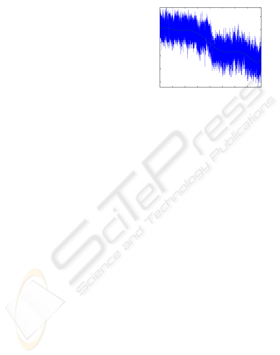
assessed the measurement error of the sensor. That
is, we evaluated the measurement precision for a still
object in order to develop a baseline performance ref-
erence. From the manufacturer specifications, the ac-
curacy is ± 2%. The precision is not specified. To
evaluate the camera’s precision, we captured thermo-
graphic images of a wood tabletop from a fixed point
of view continuously (at 27 frames/s) for approxi-
mately 30 minutes in a room at about 24
◦
C. The
room temperature was not controlled. We selected
an area of 20 × 20 pixels in the middle of the im-
age. The camera was configured with a linear mea-
0 200 400 600 800 1000 1200 1400 1600
23.55
23.6
23.65
23.7
23.75
23.8
Seconds
°
C
Figure 1: Temperature measured of a tabletop during 1509
seconds, and fitted polynomial to evaluate the measurement
error.
surement range of 20
◦
C to 40
◦
C, and pixels were
quantified with 8 bits. That is, pixel values of 0 and
255 correspond to temperatures of 20
◦
C and 40
◦
C, re-
spectively. This range provides a reasonable interval
around the expected rat body temperature of approxi-
mately 30
◦
C. The interval between two adjacent pixel
values is 0.078
◦
C. Without averaging a pixel region,
the precision should be one-half of this interval, that
is 0.039
◦
C. By averaging over a region, we may ob-
tain a precision slightly better. The temperature of
the tabletop in each frame is estimated by calculat-
ing the mean of the 10 hottest pixels in the region
of interest. We computed the regression of the data
using a 7
th
order polynomial and computed the av-
erage fitting error. We used regression because the
temperature of the tabletop is not controlled and we
assume that it changes smoothly. The average pre-
cision is the average fitting error, which is 0.021
◦
C
with a standard deviation of 0.026
◦
C. Figure 1 shows
the measured temperature and the fitted polynomial.
We did not validate the accuracy as we do not have
the equipment to do so. In our measurements, we are
only interested in the temperature variation, not in its
absolute value. However, in a previous work with the
same camera, the accuracy was evaluated to 0.13
◦
C
(Camenzind et al., 2006). From the same study, the
drift is said to be negligible.
To acquire thermographic images during animal
experiments, the rat is placed in a metal mesh cubic
cage with an open top (see figure 2) and the thermo-
graphic camera is angled down toward the cage. The
usual plexiglas cage cannot be used as this material
almost totally reflects the heat radiation of the rat and
it is not visible thru it. Furthermore, heat reflections
from the rat are also visible on the side walls. Metal
mesh walls do not cause this effect. The camera is
on a 525MV tripod (Manfrotto, Bassano del Grappa
THERMOGRAPHIC BODY TEMPERATURE MEASUREMENT USING A MEAN-SHIFT TRACKER
19
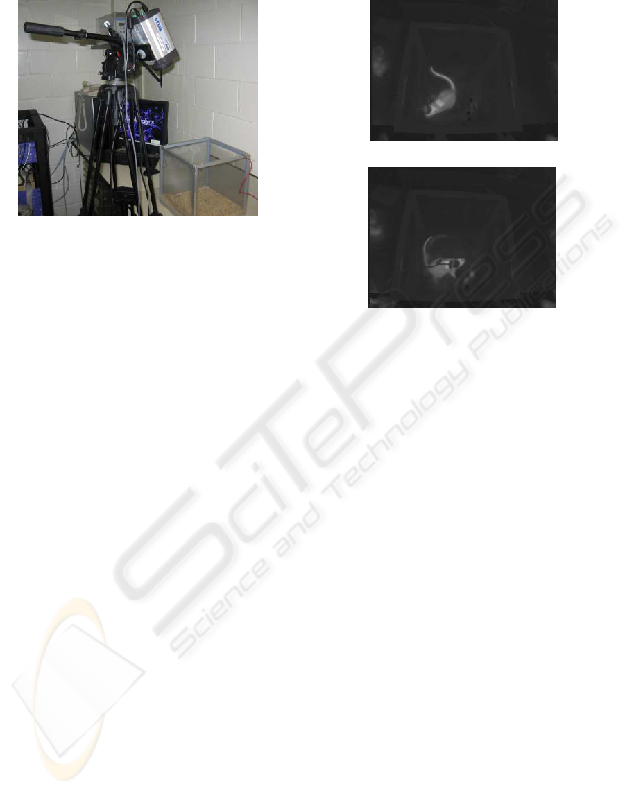
Figure 2: Camera setup and mesh cage.
(VI), Italy) and pointed toward the open top of the
cage with an angle around 20
◦
with the vertical.
During initial experiments, we quicklydetermined
that the rat fur prevented precise measurements of
the body temperature. Temperature measures on the
whole body are not reliable as they depend on the
thickness of the fur and visible area. We concluded
that the rat should have an area of approximately 10
cm
2
that is shaved to measure precisely its tempera-
ture. Indeed, the head of the rat, another interesting
region, which is warmer because it has less fur, is not
always visible and it is occluded by a device (Neural-
ynx Cheetah System, Bozeman, MT, USA) to record
local field potentials (LFP) signal on the head of the
rat. Observing the rat from the top and shaving a re-
gion on its back give better results, as this region is
almost constantly visible since the rat tends to remain
on its four feet. However, using this strategy means
that we have to use a tracking algorithm to follow the
shaved patch and discriminate it from the head. Fig-
ure 3 shows typical frames that must be processed.
The shaved patch is sometimes severely occluded by
the LFP recording device.
2.2 Measurement Area Tracking
Given the experimental setup and the measurement
strategy, computer vision is needed to track the area
for which we wish to measure temperature. Our work
is based on the following assumptions:
• the images are grayscale, with white (255) mean-
ing hot, and black (0) meaning cold in a given
range;
• the temperature of the rat is higher than its sur-
rounding,particularlyforthe shaved patch and the
head;
• the shaved patch can be occluded by the LFP
(a)
(b)
Figure 3: Two frames of shaved patch to track. (a) With-
out occlusion, (b) with occlusion from the LFP recording
device.
recording device on the head of the rat;
• the rat is always in the camera field of view.
Based on these assumptions, we have devised a
tracking method. Ideally, to get automatic measure-
ment for the complete duration of a video, the track-
ing algorithm must not loose track of the patch, and
it must not be distracted by other hot areas like the
head, which may be at a different temperature. For
tracking, we have implemented a Mean-Shift tracker
(Comaniciu et al., 2003).
Our Mean-Shift tracker follows an initially man-
ually selected area. To model the area, we assume
that the temperature inside the patch is mostly similar
for all pixels, and that the area is hotter than the sur-
rounding fur. Hence, a complex kernel and color or
texture modeling is not necessary and, in practice, do
not improve performance. Instead, we use a uniform
kernel and we calculate the probability density func-
tion (pdf) of the pixels with (x,y) coordinates inside
the area A using an histogram with n bins with
Temperature
pd f
(n) = |(x, y)|A(x, y) = n|. (1)
This histogram gives the weight w(x,y) =
Temperature
pd f
(i) of a pixel at coordinates (x,y) in
the area A with a value of i. The weight is equal to
the probability of a given pixel value estimated by the
number of its occurrence. Since most pixels have the
same values, the pixels of the shaved patch have much
BIOSIGNALS 2009 - International Conference on Bio-inspired Systems and Signal Processing
20

larger weights compared to the surrounding fur. For
each new frame, the histogram is back-projected in
the candidate area, and the Mean-Shift procedure is
applied. After convergence, we estimate the tempera-
ture based on the mean value of the hottest pixels. The
tracking algorithm can be summarized as follows:
1. Initialisation. Manually select the shaved patch
and compute the histogram of the selected area A
of size A
size
.
For each new frame f :
2. Back-project the histogram in the search area A;
that is replace a pixel value i at position (x,y)
with its number of occurrences in the histogram
(w(x,y) = Temperature
pd f
(i)).
3. Compute the location (x
c
,y
c
) of the mean weight
in the search area using the Mean-Shift procedure
with
x
c
=
∑
x
∑
y
x× w(x,y)
∑
x
∑
y
w(x,y)
(2)
and
y
c
=
∑
x
∑
y
y× w(x,y)
∑
x
∑
y
w(x,y)
. (3)
4. Center the search area at (x
c
,y
c
).
5. Repeat steps 2, 3 and 4 until convergence. That
is (x
c
,y
c
) changes by a value V
c
less than a given
threshold.
6. Calculate the temperature T
A
in the search area A
at frame f with
T
A
( f) = T
min
+ ((mean(A)/255) ∗ (T
max
− T
min
))
(4)
where T
min
and T
max
are the minimum and maxi-
mum value of the temperature range selected for
the camera.
The tracking algorithm follows an area that in-
cludes more pixels with values that have occurred
very often in the selected region in step 1. Since
the patch is about of constant temperature, the tracker
should follow it continuously. This assumption is val-
idated in the next section.
3 EXPERIMENTATION
In this section, we present the experimentation
methodology, results, and a discussion.
3.1 Experimentation Methodology
To test our measurement method, we have shot a 1h57
video of a Sprague-Dawleyrat(Charles River Labora-
tories, St-Constant, Qu´ebec, Canada) duringan exper-
imentation using 6 mg/kg i.p. of kainic acid (Sigma-
Aldrich Canada Ltd, Oakville, Ontario, Canada). All
experimental procedures conformed to institutional
policies and guidelines (Sainte-Justine Research Cen-
ter, Universit´e de Montr´eal, Qu´ebec, Canada).
The camera setup was described in section 2.1.
The video has 90706 frames at 12.89 frame per sec-
ond with a 320 × 240 resolution and compressed
with Xvid FFDshow encoder (Quality: 100%)
(http://sourceforge.net/projects/ffdshow). The video
was then processed with the Mean-Shift tracking al-
gorithm implemented in Matlab (The MathWorks,
Natick, MA, USA). We used 64 uniformbins (n = 64)
for the histogram. For convergence, we used 0.5 pixel
(V
c
= 0.5). Temperature calculations were based on
the 10 hottest pixels in the tracked area. T
min
was 20
and T
max
was 40. The size of A was A
size
= 30 (i.e.
30× 30 pixels).
Since we have a large quantity of data, to measure
the performance of our tracking algorithm we used
two metrics. For the first metric, we generated a par-
tial ground truth by selecting frames at random over
the whole video sequence. The four corners of the
patch were selected to build a bounding polygon and
the temperature value was calculated as in equation 4.
This gives a set of groundtruth temperatures T
GT
. We
selected F (F = 450) frames. The temperature mea-
surements by the tracking algorithm for these frames
were then compared with the ground truth. The eval-
uation metric is the root mean square error defined as
T
rms
=
s
1
F
F
∑
i=1
(T
A
(i) − T
GT
(i))
2
. (5)
The second metric is based on the assumption that
the temperature of the rat’s body changes smoothly.
We computed the regression of the temperatures us-
ing a 23
rd
order polynomial (largest well-conditioned
polynomial). Then, we compute the fitting error. This
gives the average precision µ
m
and its standard devi-
ation σ
m
. This fitting error is then compared with the
fitting error obtained for a static target (a tabletop, see
section 2.1) and for the ground truth. If tracking is
good, we expect the average precision (fitting error)
values to be of the same magnitude. That is, we ex-
pect a similar precision in the measurement.
THERMOGRAPHIC BODY TEMPERATURE MEASUREMENT USING A MEAN-SHIFT TRACKER
21
1000 2000 3000 4000 5000 6000 7000
0
0.2
0.4
0.6
Seconds
°
C
b)
1000 2000 3000 4000 5000 6000 7000
29
30
31
32
33
34
Seconds
°
C
a)
1000 2000 3000 4000 5000 6000 7000
29
30
31
32
33
34
c)
Seconds
°
C
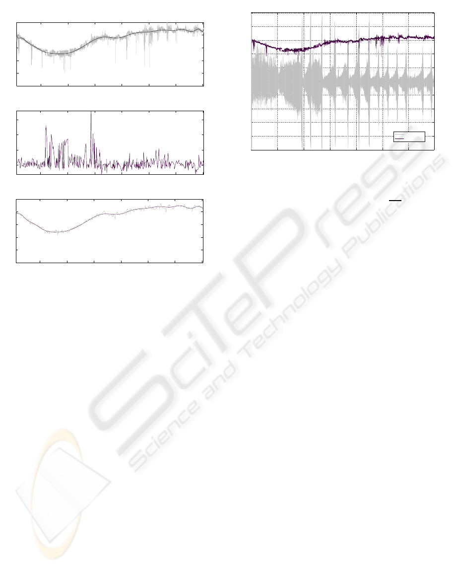
Figure 4: Results from our tracker compared to ground
truth. a) Temperature values obtained with our Mean-Shift
tracker and regression result. b) Errors for the 450 ground
truth points. c) Ground truth temperature values and regres-
sion result.
3.2 Results and Discussion
Figure 4 shows the results obtained for our test video.
The global decrease of the temperature between 0
and about 1800 seconds is caused by the kainic acid.
This phenomenon was previously observed (Ahlenius
et al., 2002) with a rectal thermometer at 15-30 min-
utes intervals. The local changes in temperature ob-
served from 3000 seconds up to the end seem to be
correlated with some seizure events (see figure 5).
This needs to be investigated further and with more
experiments.
By comparing figure 4a) and figure 4c), one can
notice that the tracker result is noisier then the ground
truth. Sudden drops of temperature of more than 1
◦
C
are caused by tracking errors or occlusions. For ex-
ample, at around 150, 1850, 2100, 4850 and 5100
seconds, the measure is not accurate because of occlu-
sion by the LFP recording device. In such cases, only
a portion of the patch is clearly visible. Sometimes
(e.g., at around 650, 4850 and 5700 seconds), the
tracker is distracted by the rat’s head. The head being
at a different temperature (also depending on its vis-
ibility) it causes a drop in the measured temperature.
1000 2000 3000 4000 5000 6000
−10
−8
−6
−4
−2
0
2
4
6
8
10
time (s)
z−scores (σ) / Temperature (
°
C)
Intensity
Temperature
Figure 5: Results from our tracker synchonized with LFP
recordings. Temperatures were shifted by -27
◦
C. The LFP
recordings were normalized around a mean µ of 0 and a
standard deviation σ of 1 (Z-scores: z =
x−µ
σ
). Z-scores
larger than ±2σ correspond to seizure events.
Other tracking errors are caused by the frame rate. In
this experiment, the frame rate was only 12.89 frames
per second because the thermographic images were
captured simultaneously with visible images from a
high resolution camera on the same computer. This
low frame rate causes tracking errors when the rat
moves too quickly because it results in a large dis-
placement in the image. In this experiment, it is the
case for the typical wet dog shakes (at about 3800,
4200, 4550, 5350, 6000, 6050 and 6700 seconds)
that follows some seizures. Note that the tempera-
ture measures are not filtered to remove outlier data.
Figure 4b) shows that the errors are mostly positive
with respect to the ground truth. This is because the
tracking errors are caused by erroneously tracking the
head which is slightly warmer than the shaved patch.
Some negative errors are not represented on this graph
since the ground truth is composed of points selected
at random and do not include all the tracking errors.
Table 1 gives the values obtained for the met-
rics defined in section 3.1. First, if we consider the
root mean square error (RMS), our mean-shift tracker
with A
size
= 30 has a value of 0.107
◦
C. This means
that, compared to ground truth, we have an error of
approximately 0.1
◦
C. The impact of this error de-
pends on the temperature changes caused by inter-
esting seizure-related phenomena. If we consider our
tracker with other parameters, using a smaller region
(A
size
= 10) than the shaved patch gives a larger RMS
error. This is because the region is smaller than many
spatial instantaneous position changes of the patch.
Thus, the patch is not in the tracker region of interest
and hence Mean-Shift does not converge to its center.
This results in a measurement area that is often not on
the patch. A
size
should be at least as large as the mo-
BIOSIGNALS 2009 - International Conference on Bio-inspired Systems and Signal Processing
22

Table 1: Average precision and root mean square error for
each method and for the still object of section 2.1. µ
m
: av-
erage precision, σ
m
: standard deviation, T
rms
: root mean
square error.
Method µ
m
(σ
m
) (
◦
C) T
rms
(
◦
C)
Still object (section 2.1) 0.021(0.026)
Ground truth 0.079(0.100) 0.000
Mean-Shift A
size
= 10 1.212(1.661) 4.601
Mean-Shift A
size
= 20 0.093(0.159) 0.110
Mean-Shift A
size
= 30 0.090(0.129) 0.107
Mean-Shift A
size
= 40 0.094(0.140) 0.144
tion of the center of the shaved area. If A
size
is selected
too large, the tracker will be distracted very often by
the head of the rat. Thus, the measurement is not reli-
able (A
size
= 40). Recall that the head is not a good re-
gion to track becauseit suffers morefrom LPF record-
ing device occlusion and from occlusions by the rat’s
body. Furthermore, when the tracker jumps from the
patch to the head, there is a measurement error since
they are not at the same temperature.
Table 1 also gives the average precision and stan-
dard deviation based on a regression with a polyno-
mial assuming smooth changes in temperature. Com-
pared to ground truth, our Mean-Shift tracker with
A
size
= 30 has an average precision about 15% larger
and standard deviation about 30% larger. Precision is
not too far from the ground truth data, but measures
are noisier because of tracking errors. Interestingly,
the ground truth precision is larger than the average
precision obtained for a still object. At this point, we
may hypothesize that it is because the shaved area is
deformable and its normal is not always aligned with
the camera sensor’s normal. Hence, the infrared radi-
ation measured by the camera changes with the angle
of the shaved area. Furthermore, as the shaved area
is deformable, the skin thickness may vary regularly
as it stretches depending on the rat position and atti-
tude. Another possibility is that seizure events cause
temperature changes that violate the smoothness con-
straints and increase the fitting error. We will test a rat
in a control condition (without kainic acid) to verify
the attainable precision with a moving target. Given
these results with our equipment, capture setup, and
assuming smooth temperature change, we can expect
to observe phenomena that cause sudden temperature
changes over a few frames larger than 0.2
◦
C.
Tracking results couldbe improvedtowardground
truth by either improving tracking or by filtering the
temperature values. To improve tracking, the focus
should be to reduce distraction by other warm areas
such as the head. This could be accomplished by ac-
counting for the trajectory of the shaved patch and us-
ing a smoothness constraint. Severe occlusions and
large position changes could be filtered using the pre-
Table 2: Computation times of the Mean-Shift tracker for
the test video sequence (1h57, 90706 frames).
Method Time (s) Frames/s
Mean-Shift A
size
= 10 16100 5.6
Mean-Shift A
size
= 20 15854 5.7
Mean-Shift A
size
= 30 16365 5.5
Mean-Shift A
size
= 40 16087 5.6
vious and following frames over a time window. A
higher frame rate would also reduce the occurrence
of large position changes.
Table 2 shows the computation times required to
process the whole test sequence using MATLAB on
a Opteron 250 2.4 GHz computer (Advanced Mi-
cro Devices, Sunnyvale, CA, USA). We can process
approximately 5.6 frames/s. The processing time is
mostly constant for the tested values of A
size
. This is
because the processing time is related to convergence
of the Mean-Shift procedure (step 5 in section 2.2)
more than to processing a larger number of pixels in
area A.
4 CONCLUSIONS
This paper presented a methodology to measure the
body temperature of a moving animal in a laboratory
setting. Because of the experimental setup, uneven
thickness of the fur with viewpoint and the possibil-
ity of occlusion, we have concluded that we needed
to shave a region on the back of the rat. Since the
head and this shaved region can have different tem-
peratures, tracking is required to measure temperature
on the same body region continuously. We proposed
a Mean-Shift tracker based on the probability density
function of the temperature of a manually selected
area.
Our method was tested on a 2-hour video se-
quence with a rat having seizures at regular intervals.
Results show that our tracker achieves measurements
with an RMS error of 0.1
◦
C. Errors are caused by se-
vere occlusions or by distracting warm regions such
as the head. Although we estimate we can observe
phenomena causing changes of more than 0.2
◦
C, we
do not obtain a precision similar to a still object. Part
of this difference with camera precision is caused by
the tracker, while another part is caused by other rea-
sons. We hypothesize that changes in the orientation
of the measured surface cause measurement errors, so
it may not be possible to attain the precision obtained
on a still object. Furthermore, in the test video, tem-
perature changes may not be smooth and they may
increase the fitting error by a polynomial.
THERMOGRAPHIC BODY TEMPERATURE MEASUREMENT USING A MEAN-SHIFT TRACKER
23

Future works include the improvement of the
tracking algorithm by adding trajectory smoothness
constraints. That is, the change in position in the im-
age of the tracked area should be smooth. Further-
more, filtering will be applied to the temperature mea-
sures to remove outliers. We will also investigate the
impact of changes of orientation of the measured sur-
face. Finally, we want to apply this methodology in
more experiments and automatically detect abnormal
events based on changes in the body temperature.
ACKNOWLEDGEMENTS
We would like to thank the Canada Foundation for
Innovation (CFI) for their support (grant 10420).
REFERENCES
Ahlenius, S., Oprica, M., Eriksson, C., Winblad, B., and
Schultzberg, M. (July 2002). Effects of kainic acid
on rat body temperature: unmasking by dizocilpine.
Neuropharmacology, 43(1):28–35.
Amalu, W. (2004). Nondestructive testing of the hu-
man breast: the validity of dynamic stress testing in
medical infrared breast imaging. In Engineering in
Medicine and Biology Society, 2004. IEMBS ’04. 26th
Annual International Conference of the IEEE, vol-
ume 2, pages 1174–1177.
Camenzind, M., Weder, M., Rossi, R., and Kowtsch, C.
(2006). Remote sensing infrared thermography for
mass-screening at airports and public events: Study to
evaluate the mobile use of infrared cameras to identify
persons with elevated body temperature and their use
for mass screening. Technical Report 204991, EMPA
Materials Science and Technology.
Carmant, L. (2006). Mechanisms that might underlie pro-
gression of the epilepsies and how to potentially alter
them. Advances in neurology, 97:305–314.
Celka, P. and Colditz, P. (May 2002). A computer-aided de-
tection of eeg seizures in infants: a singular-spectrum
approach and performance comparison. Biomedical
Engineering, IEEE Transactions on, 49(5):455–462.
Comaniciu, D., Ramesh, V., and Meer, P. (May 2003).
Kernel-based object tracking. Pattern Analysis
and Machine Intelligence, IEEE Transactions on,
25(5):564–577.
Faul, S., Boylan, G., Connolly, S., Marnane, L., and Light-
body, G. (July 2005). An evaluation of automated
neonatal seizure detection methods. Clinical Neuro-
physiology, (7):1533–1541.
Karayiannis, N., Srinivasan, S., Bhattacharya, R., Wise,
M., Frost, J.D., J., and Mizrahi, E. (Sep 2001). Ex-
traction of motion strength and motor activity signals
from video recordings of neonatal seizures. Medical
Imaging, IEEE Transactions on, 20(9):965–980.
Karayiannis, N., Tao, G., Frost, J.D., J., Wise, M.,
and Mizrahi, E. (July 2006). Automated detec-
tion of videotaped neonatal seizures based on mo-
tion segmentation methods. Clinical Neurophysiol-
ogy, (7):1585–1594.
Sunderam, S. and Osorio, I. (August 2003). Mesial tempo-
ral lobe seizures may activate thermoregulatory mech-
anisms in humans: an infrared study of facial temper-
ature. Epilepsy and Behavior, 49(4):399–406.
Volpe, J. J. (1989). Neonatal Seizures: Current Concepts
and Revised Classification. Pediatrics, 84(3):422–
428.
BIOSIGNALS 2009 - International Conference on Bio-inspired Systems and Signal Processing
24
