A NEW REINFORCEMENT SCHEME FOR STOCHASTIC
LEARNING AUTOMATA
Application to Automatic Control
Florin Stoica, Emil M. Popa
Computer Science Department, “Lucian Blaga” University, Str. Dr. Ion Ratiu 5-7, Sibiu, Romania
Iulian Pah
Department of Sociology, “Babes-Bolyai” University, Bd.21 decembrie 1989, no.128-130, Cluj-Napoca, Romania
Keywords: Stochastic Learning Automata, Reinforcement Learning, Intelligent Vehicle Control, agents.
Abstract: A Learning Automaton is a learning entity that learns the optimal action to use from its set of possible
actions. It does this by performing actions toward an environment and analyzes the resulting response. The
response, being both good and bad, results in behaviour change to the automaton (the automaton will learn
based on this response). This behaviour change is often called reinforcement algorithm. The term stochastic
emphasizes the adaptive nature of the automaton: environment output is stochastically related to the
automaton action. The reinforcement scheme presented in this paper is shown to satisfy all necessary and
sufficient conditions for absolute expediency for a stationary environment. An automaton using this scheme
is guaranteed to „do better” at every time step than at the previous step. Some simulation results are
presented, which prove that our algorithm converges to a solution faster than one previously defined in
(Ünsal, 1999). Using Stochastic Learning Automata techniques, we introduce a decision/control method for
intelligent vehicles, in infrastructure managed architecture. The aim is to design an automata system that can
learn the best possible action based on the data received from on-board sensors or from the localization
system of highway infrastructure. A multi-agent approach is used for effective implementation. Each
vehicle has associated a “driver” agent, hosted on a JADE platform.
1 INTRODUCTION
The past and present research on vehicle control
emphasizes the importance of new methodologies in
order to obtain stable longitudinal and lateral
control. In this paper, we consider stochastic
learning automata as intelligent controller within our
model for an Intelligent Vehicle Control System.
An automaton is a machine or control
mechanism designed to automatically follow a
predetermined sequence of operations or respond to
encoded instructions. The term stochastic
emphasizes the adaptive nature of the automaton we
describe here. The automaton described here does
not follow predetermined rules, but adapts to
changes in its environment. This adaptation is the
result of the learning process (Barto, 2003).
Learning is defined as any permanent change in
behavior as a result of past experience, and a
learning system should therefore have the ability to
improve its behavior with time, toward a final goal.
The stochastic automaton attempts a solution of
the problem without any information on the optimal
action (initially, equal probabilities are attached to
all the actions). One action is selected at random, the
response from the environment is observed, action
probabilities are updated based on that response, and
the procedure is repeated. A stochastic automaton
acting as described to improve its performance is
called a learning automaton. The algorithm that
guarantees the desired learning process is called a
reinforcement scheme (Moody, 2004).
Mathematically, the environment is defined by a
triple
},,{
β
α
c where },...,,{
21 r
α
α
α
α
=
represents
a finite set of actions being the input to the
environment,
},{
21
β
β
β
=
represents a binary
response set, and
},...,,{
21 r
cccc
=
is a set of penalty
45
Stoica F., M. Popa E. and Pah I. (2008).
A NEW REINFORCEMENT SCHEME FOR STOCHASTIC LEARNING AUTOMATA - Application to Automatic Control.
In Proceedings of the International Conference on e-Business, pages 45-50
DOI: 10.5220/0001909800450050
Copyright
c
 SciTePress

probabilities, where
i
c is the probability that action
i
α
will result in an unfavorable response. Given that
0)( =n
β
is a favorable outcome and 1)(
=
n
β
is an
unfavorable outcome at time instant
...),2,1,0( =nn , the element
i
c of
c
is defined
mathematically by:
rinnPc
ii
...,,2,1))(|1)(( ====
α
α
β
The environment can further be split up in two
types, stationary and nonstationary. In a stationary
environment the penalty probabilities will never
change. In a nonstationary environment the penalties
will change over time.
In order to describe the reinforcement schemes,
is defined
)(np , a vector of action probabilities:
rinPnp
ii
,1),)(()( === αα
Updating action probabilities can be represented
as follows:
)](),(),([)1( nnnpTnp
β
α
=+
where T is a mapping. This formula says the next
action probability
)1( +np is updated based on the
current probability
)(np , the input from the
environment and the resulting action. If
)1(
+
np is a
linear function of
)(np , the reinforcement scheme is
said to be linear; otherwise it is termed nonlinear.
2 REINFORCEMENT SCHEMES
2.1 Performance Evaluation
Consider a stationary random environment with
penalty probabilities
},...,,{
21 r
ccc defined above.
We define a quantity
)(nM as the average
penalty for a given action probability vector:
∑
=
=
r
i
ii
npcnM
1
)()(
An automaton is absolutely expedient if the
expected value of the average penalty at one
iteration step is less than it was at the previous step
for all steps:
)()1( nMnM <+ for all
n
(Rivero,
2003)
.
The algorithm which we will present in this
paper is derived from a nonlinear absolutely
expedient reinforcement scheme presented by
(Ünsal, 1999).
2.2 Absolutely Expedient
Reinforcement Schemes
The reinforcement scheme is the basis of the
learning process for learning automata. The general
solution for absolutely expedient schemes was found
by (Lakshmivarahan, 1973).
A learning automaton may send its action to
multiple environments at the same time. In that case,
the action of the automaton results in a vector of
responses from environments (or “teachers”). In a
stationary N-teacher environment, if an automaton
produced the action
i
α
and the environment
responses are
Nj
j
i
,...,1= β at time instant n , then
the vector of action probabilities
)(np is updated as
follows (
Ünsal, 1999):
∑∑
≠
==
−∗
⎥
⎦
⎤
⎢
⎣
⎡
+=+
r
ij
j
j
N
k
k
iii
np
N
npnp
11
))((
1
)()1( φβ
∑∑
≠
==
∗
⎥
⎦
⎤
⎢
⎣
⎡
−−
r
ij
j
j
N
k
k
i
np
N
11
))((
1
1 ψβ
))((
1
1
))((
1
)()1(
1
1
np
N
np
N
npnp
j
N
k
k
i
j
N
k
k
ijj
ψβ
φβ
∗
⎥
⎦
⎤
⎢
⎣
⎡
−+
+∗
⎥
⎦
⎤
⎢
⎣
⎡
−=+
∑
∑
=
=
for all
ij
≠
where the functions
i
φ
and
i
ψ
satisfy
the following conditions:
))((
)(
))((
...
)(
))((
1
1
np
np
np
np
np
r
r
λ
φφ
=== (2)
))((
)(
))((
...
)(
))((
1
1
np
np
np
np
np
r
r
μ
ψψ
===
∑
≠
=
>+
r
ij
j
ji
npnp
1
0))(()( φ (3)
∑
≠
=
<−
r
ij
j
ji
npnp
1
1))(()( ψ (4)
0))(()( >
+
npnp
jj
ψ
(5)
1))(()(
<
−
npnp
jj
φ
(6)
for all }{\},...,1{ irj
∈
The conditions (3)-(6) ensure that
rkp
k
,1,10 =<< (Stoica, 2007).
Theorem. If the functions
))(( np
λ
and ))(( np
μ
satisfy the following conditions:
(1)
ICE-B 2008 - International Conference on e-Business
46

0))(( ≤np
λ
0))(( ≤np
μ
(7)
0))(())(( <+ npnp
μ
λ
then the automaton with the reinforcement scheme
in (1) is absolutely expedient in a stationary
environment.
The proof of this theorem can be found in (
Baba,
1984
).
3 A NEW NONLINEAR
REINFORCEMENT SCHEME
Because the above theorem is also valid for a single-
teacher model, we can define a single environment
response that is a function
f of many teacher
outputs.
Thus, we can update the above algorithm as
follows:
)](1[)()1(
)](1[))(()()1(
npf
npnHfnpnp
i
iii
−∗−∗−−
−−∗∗∗−∗+=+
θ
δθ
)()()1()(
))(()()1(
npfnp
nHfnpnp
jj
jj
∗−∗−+∗
∗∗∗−∗−=+
θ
δθ
(8)
for all
ij ≠ , i.e.:
)())(( npnp
kk
∗
−
=
θ
ψ
)()())(( npnHnp
kk
∗∗∗−=
δ
θ
φ
where learning parameters
θ
and
δ
are real values
which satisfy:
10 <<
θ
and 10 <∗<
δ
θ
.
The function
H
is defined as follows:
{{
⎩
⎨
⎧
−
−∗∗
= ,
))(1(
)(
minmax;1min)(
ε
δθ
np
np
nH
i
i
}}
0;
)(
)(1
,1
⎪
⎭
⎪
⎬
⎫
⎟
⎟
⎠
⎞
⎜
⎜
⎝
⎛
−
∗∗
−
≠
=
ij
rj
j
j
np
np
ε
δθ
Parameter
ε
is an arbitrarily small positive real
number.
Our reinforcement scheme differs from the one
given in (
Ünsal, 1999) by the definition of these
two functions:
H
and
k
φ
.
The proof that all the conditions of the
reinforcement scheme (1) and theorem (7) are
satisfied can be found in (Stoica, 2007).
In conclusion, we state the algorithm given in
equations (8) is absolutely expedient in a stationary
environment.
4 EXPERIMENTAL RESULTS
4.1 Problem Formulation
To show that our algorithm converges to a solution
faster than the one given in (Ünsal, 1999), let us
consider a simple example. Figure 1 illustrates a grid
world in which a robot navigates. Shaded cells
represent barriers.
Figure 1: A grid world for robot navigation.
The current position of the robot is marked by a
circle. Navigation is done using four actions
},,,{ WESN
=
α
, the actions denoting the four
possible movements along the coordinate directions.
Because in given situation there is a single
optimal action, we stop the execution when the
probability of the optimal action reaches a certain
value (0.9999).
4.2 Comparative Results
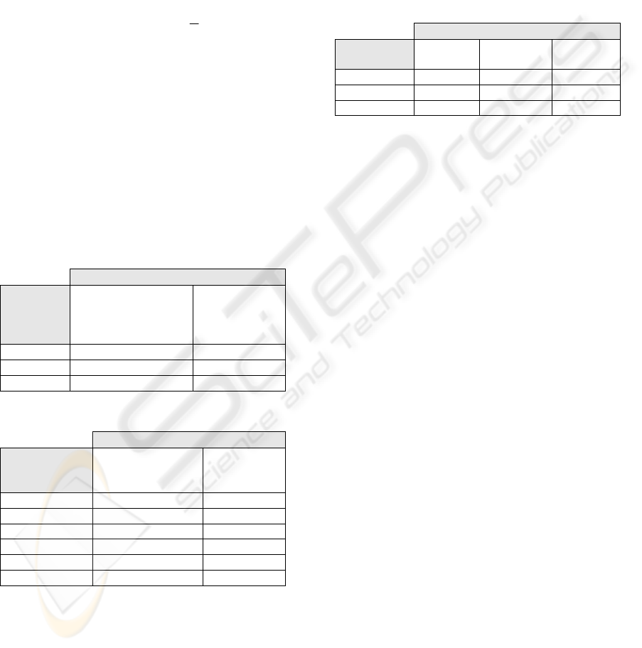
We compared two reinforcement schemes using
these four actions and two different initial
conditions.
Table 1: Convergence rates for a single optimal action of a
4-action automaton (200 runs for each parameter set).
Average number of steps to reach
p
o
p
t
=0.9999
4 actions with
4,1
,4/1)0(
=
=
i
p
i
4 actions with
3/9995.0
,0005.0)0(
=
=
≠opti
opt
p
p
θ
δ
Ünsal’s
Alg.
New
alg.
Ünsal’s
Alg.
New
alg.
0.01
1 644.84 633.96 921.20 905.18
25 62.23 56.64 205.56 194.08
50 11.13 8.73 351.67 340.27
0.05
1 136.99 130.41 202.96 198.25
5 74.05 63.93 88.39 79.19
10 24.74 20.09 103.21 92.83
0.1
1 70.81 63.09 105.12 99.20
2.5 59.48 50.52 71.77 65.49
5 23.05 19.51 59.06 54.08
The data shown in Table 1 are the results of two
different initial conditions where in first case all
A NEW REINFORCEMENT SCHEME FOR STOCHASTIC LEARNING AUTOMATA - Application to Automatic
Control
47

probabilities are initially the same and in second
case the optimal action initially has a small
probability value (0.0005), with only one action
receiving reward (i.e., optimal action).
Comparing values from corresponding columns,
we conclude that our algorithm converges to a
solution faster than the one given in (Ünsal, 1999).
5 USING STOCHASTIC
LEARNING AUTOMATA FOR
INTELLIGENT VEHICLE
CONTROL
The task of creating intelligent systems that we can
rely on is not trivial. In this section, we present a
method for intelligent vehicle control, having as
theoretical background Stochastic Learning
Automata. We visualize the planning layer of an
intelligent vehicle as an automaton (or automata
group) in a nonstationary environment. We attempt
to find a way to make intelligent decisions here,
having as objectives conformance with traffic
parameters imposed by the highway infrastructure
(management system and global control), and
improved safety by minimizing crash risk.
The aim here is to design an automata system
that can learn the best possible action based on the
data received from on-board sensors, of from
roadside-to-vehicle communications. For our model,
we assume that an intelligent vehicle is capable of
two sets of lateral and longitudinal actions. Lateral
actions are LEFT (shift to left lane), RIGHT (shift to
right lane) and LINE_OK (stay in current lane).
Longitudinal actions are ACC (accelerate), DEC
(decelerate) and SPEED_OK (keep current speed).
An autonomous vehicle must be able to “sense” the
environment around itself. Therefore, we assume
that there are four different sensors modules on
board the vehicle (the headway module, two side
modules and a speed module), in order to detect the
presence of a vehicle traveling in front of the vehicle
or in the immediately adjacent lane and to know the
current speed of the vehicle.
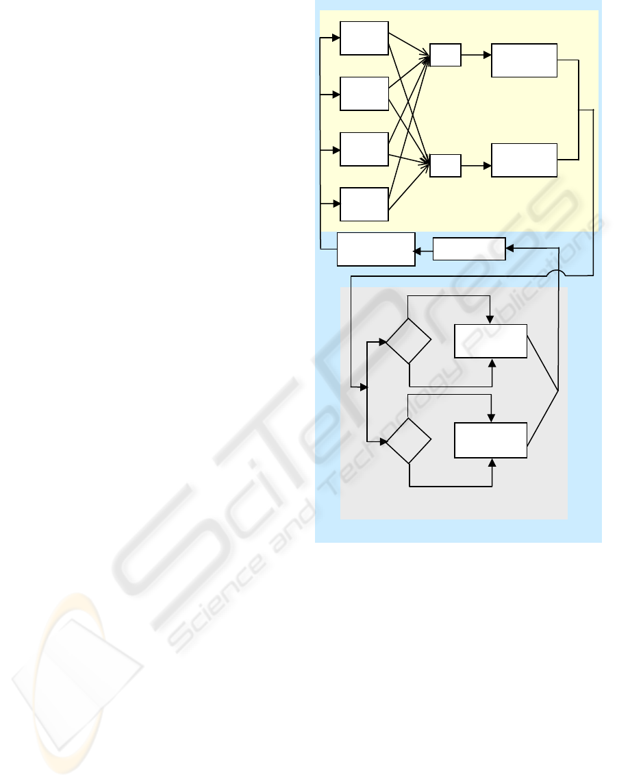
These sensor modules evaluate the information
received from the on-board sensors or from the
highway infrastructure in the light of the current
automata actions, and send a response to the
automata. Our basic model for planning and
coordination of lane changing and speed control is
shown in Figure 2.
Figure 2: The model of the Intelligent Vehicle Control
System.
The response from physical environment is a
combination of outputs from the sensor modules.
Because an input parameter for the decision blocks
is the action chosen by the stochastic automaton, is
necessary to use two distinct functions
1
F and
2
F
for mapping the outputs of decision blocks in inputs
for the two learning automata, namely the
longitudinal automaton and respectively the lateral
automaton.
After updating the action probability vectors in
both learning automata, using the nonlinear
reinforcement scheme presented in section 3, the
outputs from stochastic automata are transmitted to
the regulation layer. The regulation layer handles
the actions received from the two automata in a
distinct manner, using for each of them a regulation
Physical Environment
Auto
vehicle
SLA
Environment
Planning Layer
0
2
= β
Frontal
Detection
Left
Detection
Right
Detection
Speed
Detection
F1
F2
Longitudina
l
Lateral
Automaton
Regulation
Buffe
r
Highway
Regulation
Buffer
0
1
= β
y
es
no
y
es
no
1
β
2
β
Localization
System
1
α
2
α
1
α
2
α
1
α
2
α
─
─
action
ICE-B 2008 - International Conference on e-Business
48

buffer. If an action received was rewarded, it will be
introduced in the regulation buffer of the
corresponding automaton, else in buffer will be
introduced a certain value which denotes a penalized
action by the physical environment. The regulation
layer does not carry out the action chosen
immediately; instead, it carries out an action only if
it is recommended
k times consecutively by the
automaton, where
k is the length of the regulation
buffer. After an action is executed, the action
probability vector is initialized to
r
1
, where
r
is the
number of actions. When an action is executed,
regulation buffer is initialized also.
6 SENSOR MODULES
The four teacher modules mentioned above are
decision blocks that calculate the response
(reward/penalty), based on the last chosen action of
automaton. Table 2 describes the output of decision
blocks for side sensors.
Table 2: Outputs from the Left/Right Sensor Module.
Left/Right Sensor Module
Actions
Vehicle in sensor
range or no adjacent
lane
No vehicle in
sensor range
and adjacent
lane exists
LINE_OK 0/0 0/0
LEFT 1/0 0/0
RIGHT 0/1 0/0
Table 3: Outputs from the Headway Module.
Headway Sensor Module
Actions
Vehicle in range
(at a close frontal
distance)
No vehicle
in range
LINE_OK 1 0
LEFT 0 0
RIGHT 0 0
SPEED_OK 1 0
ACC 1 0
DEC 0* 0
As seen in Table 2, a penalty response is
received from the left sensor module when the
action is LEFT and there is a vehicle in the left or
the vehicle is already traveling on the leftmost lane.
There is a similar situation for the right sensor
module.
The Headway (Frontal) Module is defined as
shown in Table 3. If there is a vehicle at a close
distance (< admissible distance), a penalty response
is sent to the automaton for actions LINE_OK,
SPEED_OK and ACC. All other actions (LEFT,
RIGHT, DEC) are encouraged, because they may
serve to avoid a collision.
The Speed Module compares the actual speed
with the desired speed, and based on the action
choosed send a feedback to the longitudinal
automaton.
Table 4: Outputs from the Speed Module.
Speed Sensor Module
Actions
Speed:
too slow
Acceptable
speed
Speed:
too fast
SPEED_OK 1 0 1
ACC 0 0 1
DEC 1 0 0
The reward response indicated by 0* (from the
Headway Sensor Module) is different than the
normal reward response, indicated by 0: this reward
response has a higher priority and must override a
possible penalty from other modules.
7 A MULTI-AGENT SYSTEM
FOR INTELLIGENT VEHICLE
CONTROL
In this section is described an implementation of a
simulator for the Intelligent Vehicle Control System,
in a multi-agent approach. The entire system was
implemented in Java, and is based on JADE
platform (Bigus, 2001).
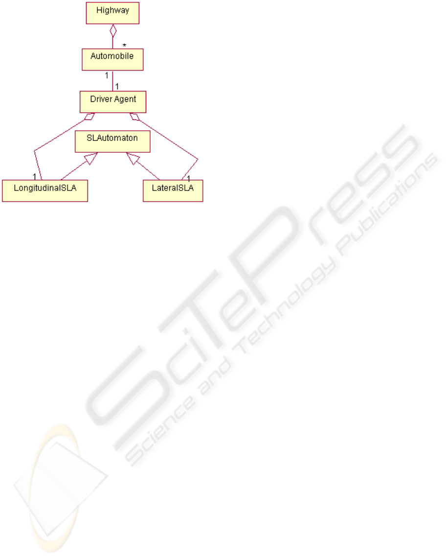
In figure 3 is showed the class diagram of the
simulator. Each vehicle has associated a JADE agent
(
DriverAgent), responsible for the intelligent control.
“Driving” means a continuous learning process,
sustained by the two stochastic learning automata,
namely the longitudinal automaton and respectively
the lateral automaton.
The response of the physical environment is a
combination of the outputs of all four sensor
modules. The implementation of this combination
for each automaton (longitudinal respectively
lateral) is showed in figure 4 (the value 0* was
substituted by 2).
A NEW REINFORCEMENT SCHEME FOR STOCHASTIC LEARNING AUTOMATA - Application to Automatic
Control
49

Figure 3: The class diagram of the simulator.
// Longitudinal Automaton
public double reward(int action){
int combine;
combine=Math.max(speedModule(action),
frontModule(action));
if (combine = = 2) combine = 0;
return combine;
}
// Lateral Automaton
public double reward(int action){
int combine;
combine=Math.max(
leftRightModule(action),
frontModule(action));
return combine;
}
Figure 4: The physical environment response.
8 CONCLUSIONS
Reinforcement learning has attracted rapidly
increasing interest in the machine learning and
artificial intelligence communities. Its promise is
beguiling - a way of programming agents by reward
and punishment without needing to specify how the
task (i.e., behavior) is to be achieved. Reinforcement
learning allows, at least in principle, to bypass the
problems of building an explicit model of the
behavior to be synthesized and its counterpart, a
meaningful learning base (supervised learning).
The reinforcement scheme presented in this
paper satisfies all necessary and sufficient conditions
for absolute expediency in a stationary environment
and the nonlinear algorithm based on this scheme is
found to converge to the ”optimal” action faster than
nonlinear schemes previously defined in (Ünsal,
1999).
Using this new reinforcement scheme was
developed a simulator for an Intelligent Vehicle
Control System, in a multi-agent approach. The
entire system was implemented in Java, and is based
on JADE platform
REFERENCES
Baba, N., 1984. New Topics in Learning Automata:
Theory and Applications, Lecture Notes in Control
and Information Sciences Berlin, Germany: Springer-
Verlag.
Barto, A., Mahadevan, S., 2003. Recent advances in
hierarchical reinforcement learning, Discrete-Event
Systems journal, Special issue on Reinforcement
Learning.
Bigus, J. P., Bigus, J., 2001. Constructing Intelligent
Agents using Java, 2nd ed., John Wiley & Sons, Inc.
Buffet, O., Dutech, A., Charpillet, F., 2001. Incremental
reinforcement learning for designing multi-agent
systems, In J. P. Müller, E. Andre, S. Sen, and C.
Frasson, editors, Proceedings of the Fifth
International Conference onAutonomous Agents, pp.
31–32, Montreal, Canada, ACM Press.
Lakshmivarahan, S., Thathachar, M.A.L., 1973.
Absolutely Expedient Learning Algorithms for
Stochastic Automata, IEEE Transactions on Systems,
Man and Cybernetics, vol. SMC-6, pp. 281-286.
Moody, J., Liu, Y., Saffell, M., Youn, K., 2004. Stochastic
direct reinforcement: Application to simple games
with recurrence, In Proceedings of Artificial
Multiagent Learning. Papers from the 2004 AAAI Fall
Symposium,Technical Report FS-04-02.
Narendra, K. S., Thathachar, M. A. L., 1989. Learning
Automata: an introduction, Prentice-Hall.
Rivero, C., 2003. Characterization of the absolutely
expedient learning algorithms for stochastic automata
in a non-discrete space of actions, ESANN'2003
proceedings - European Symposium on Artificial
Neural Networks Bruges (Belgium), ISBN 2-930307-
03-X, pp. 307-312
Stoica, F., Popa, E. M., 2007. An Absolutely Expedient
Learning Algorithm for Stochastic Automata, WSEAS
Transactions on Computers, Issue 2, Volume 6, ISSN
1109-2750, pp. 229-235.
Sutton, R., Barto, A., 1998. Reinforcement learning: An
introduction, MIT-press, Cambridge, MA.
Ünsal, C., Kachroo, P., Bay, J. S., 1999. Multiple
Stochastic Learning Automata for Vehicle Path
Control in an Automated Highway System, IEEE
Transactions on Systems, Man, and Cybernetics -part
A: systems and humans, vol. 29, no. 1, january 1999.
ICE-B 2008 - International Conference on e-Business
50