
RBF NETWORK COMBINED WITH WAVELET DENOISING FOR
SARDINE CATCHES FORECASTING
Nibaldo Rodriguez, Broderick Crawford and Eleuterio Ya˜nez
Pontificia Universidad Catolica de Valparaiso, Chile
Keywords:
Neural networks, wavelet denoising, forecasting.
Abstract:
This paper deals with time series of monthly sardines catches in the north area of Chile. The proposed method
combines radial basis function neural network (RBFNN) with wavelet denoising algorithm. Wavelet denoising
is based on stationary wavelet transform with hard thresholding rule and the RBFNN architecture is composed
of linear and nonlinear weights, which are estimated by using the separable nonlinear least square method.
The performance evaluation of the proposed forecasting model showed that a 93% of the explained variance
was captured with a reduced parsimony.
1 INTRODUCTION
In fisheries management policy the main goal is to
establish the future catch per unit of effort (CPUE)
values in a concrete area during a know period keep-
ing the stock replacements. To achieve this aim lin-
eal regression methodology has been successful in
describing and forecasting the fishery dynamics of a
wide variety of species (Stergiou, 1996) (Stergiou and
Christou, 1996). However, this technique is ineffi-
cient for capturing both nonstationary and nonlinear-
ities phenomena in sardine catch forecasting time se-
ries. Recently there has been an increased interest in
both neural networks techniques and wavelet theory
to model complex relationship in nonstationary time
series. Neural networks have been used for forecast-
ing model due to their ability to approximate a wide
range of unknown nonlinear functions (K. Hornik and
White, 1989). On the other hand, wavelet theory can
produce a local representation of a times series in both
time and frequency domain and is not restrained by
the assumption of stationary.
Gutierrez et. al. (J. Gutierrez and Pulido, 2007),
propose a forecasting model of sardine catches based
on a sigmoidal neural network, whose architecture
is composed of an input layer of 6 nodes, two hid-
den layers having 15 nodes each layer, and a lin-
ear output layer of a single node. Some disadvan-
tages of this architecture is its high parsimony as
well as computational time cost during the estima-
tion of linear and nonlinear weights. As shown in
(J. Gutierrez and Pulido, 2007), when applying the
Levenberg Marquardt (LM) algorithm (Hagan and
Menhaj, 1994), the forecasting model achieves a de-
termination coefficient of 82%. A better result of
the determination coefficient can be achieved if sig-
moidal neural network is substituted by a radial ba-
sis function neural network combined with wavelet
denoising techniques based on translation-invariant
wavelet transform. Coifman and Donoho (Coifman
and Donoho, 1995) introduced translation-invariant
wavelet denoising algorithm based on the idea of cy-
cle spinning, which is equivalent to denoising using
the discrete stationary wavelet transform (SWT) (Na-
son and Silverman, 1995) (Pesquet and Carfantan,
1995). Besides, Coifman and Donoho showed that
SWT denoising achieves better root mean squared er-
ror than traditional descrete wavelettransform denois-
ing. Therefore, we employ the SWT for denoising
monthly sardine catches data.
In this paper, we propose a RBFNN combined
with wavelet denoising algorithm for forecasting the
monthly sardine catch per unit of effort value. The
RBFNN architecture consists of two components
(Karayiannis, 1999): a linear weights subset and
a nonlinear hidden weights subset. Both compo-
nents are estimated by using the separable nonlinear
least squares (SNLS) minimization procedures (Serre,
2002). The SNLS scheme consists of two phases. In
the first phase, the hidden weights are fixed and out-
put weights are estimated with a linear least squares
method. In a second phase, the output weights are
fixed and the hidden weights are estimated using the
LM algorithm (Hagan and Menhaj, 1994). For sar-
308
Rodriguez N., Crawford B. and Yañez E. (2008).
RBF NETWORK COMBINED WITH WAVELET DENOISING FOR SARDINE CATCHES FORECASTING.
In Proceedings of the Third International Conference on Software and Data Technologies - ISDM/ABF, pages 308-311
DOI: 10.5220/0001893403080311
Copyright
c
SciTePress

dines catches forecasting, advantages of the proposed
model are reducing the parsimony, improvement of
convergence speed, and increasing accuracy preci-
sion. On the other hand, Wavelet denoising algorithm
employs the stationary wavelet transform with univer-
sal threshold rule.
The layout of this paper is as follows. In section 2,
the forecasting scheme based on both wavelet denois-
ing and RBFNN with hybrid algorithm for adjusting
the linear and nonlinear weights are presented. The
performance evaluation curves of the forecaster effect
are discussed in Section 3. Finally, the conclusions
are drawn in the last section.
2 FORECASTING MODEL
The forecasted signal s(t) can be decomposedin a low
frequency component and a high frequency compo-
nent. The low frequency component is approximated
using a autoregressive model and the high frequency
component is approximated using a RBFNN. That is,
y =
N
h
∑
j=1
b
j
φ
j
(u
k
,v
j
) +
m
∑
k=1
c
k
u
k
(1)
where N
h
is the number of hidden nodes, m is the
number input nodes, u denotes the regression vec-
tor u = (u
1
,u
2
,... u
m
) containing lagged m-values,
w = [b
0
,b
1
,... b
N
h
,c
1
,c
2
,... c
m
] are the linear output
parameters, v = [v
1
,v
2
,... v
N
h
] are the nonlinear hid-
den parameters, and φ
j
(·) are hidden activation func-
tions, which is derived as (Karayiannis, 1999)
φ
j
(u
k
) = φ(ku
k
− v
j
k
2
) (2a)
φ(λ) = (λ + 1)
−1/2
(2b)
In order to estimate the linear parameters {w
j
}
and nonlinear parameters {v
j
} of the forecaster an hy-
brid training algorithm is proposed, which is based on
least square (LS) method and Levenberg-Marquardt
(LM) algorithms. The LS algorithm is used to esti-
mate the parameters { w
j
} and the LM algorithm is
used to adapts the nonlinear parameters {v
j
}.
Now suppose a set of training input-output sam-
ples, denoted as {u
i,k
,d
i
,i = 1,.. .,N
s
,k = 1,... , m ).
Then we can perform N
s
equations of the form of (1)
as follows
Y = WΦ (3)
where the desired output d
i
and input data u
i
are
obtained as
d
i
= [
˜
s(t)] (4a)
u
i
= [
˜
s(t − 1)
˜
s(t − 2)···
˜
s(t − m)] (4b)
where
˜
s(t) represent denoised sardine catches
data. For any given representation of the nonlinear
parameters {v
j
}, the optimal values of the linear pa-
rameters { ˆw
j
} are obtained using the LS algorithm as
follows
ˆ
W = Φ
†
D (5)
where D = [d
1
d
2
··· d
N
s
] is the desired output
patter vector and Φ
†
is the Moore-Penrose general-
ized inverse (Serre, 2002) of the activation function
output matrix Φ.
Once linear parameters
ˆ
W are obtained, the LM
algorithm adapts the nonlinear parameters of the hid-
den activation functions minimizing mean square er-
ror, which is defined as
E(v) =
N
s
∑
i=1
(d
i
− y
i
)
2
(6a)
Y =
ˆ
WΦ (6b)
Finally, the LM algorithm adapts the parameter
v = [v
1
···v
Nh
] according to the following equations
(Hagan and Menhaj, 1994)
v = v+ ∆v (7a)
∆v = (JJ
T
+ αI)
−1
J
T
E (7b)
where J represent Jacobian matrix of the error
vector e(v
i
) = d
i
− y
i
evaluated in v
i
, I is the iden-
tity matrix. The error vector e(v
i
) is the error of the
RBFNN for i-patter. The parameter µ is increased or
decreased at each step.
2.1 Wavelet Denoising Algorithm
The wavelet denoising algorithm is based on three
stages: (i) the stationary wavelet transform of time
series s(t); (ii) thresholding the wavelet coefficients;
(iii) the inverse stationary wavelet transform of the
thresholding wavelet coefficients to obtain the de-
noised time series
˜
s(t).
According to the original hard thresholding rule
with the universal threshold, the wavelet coefficients
{cD
1
,cD
2
,...,cD
N
} are thresholded by the threshold
value given by (Donoho, 1995)
T = σ
p
2log(N) (8a)
σ =
median(| cD
i
|)
0.6745
(8b)
where N es the length of time series s(t) and σ is
the noise level.
RBF NETWORK COMBINED WITH WAVELET DENOISING FOR SARDINE CATCHES FORECASTING
309
3 EXPERIMENTS AND RESULTS
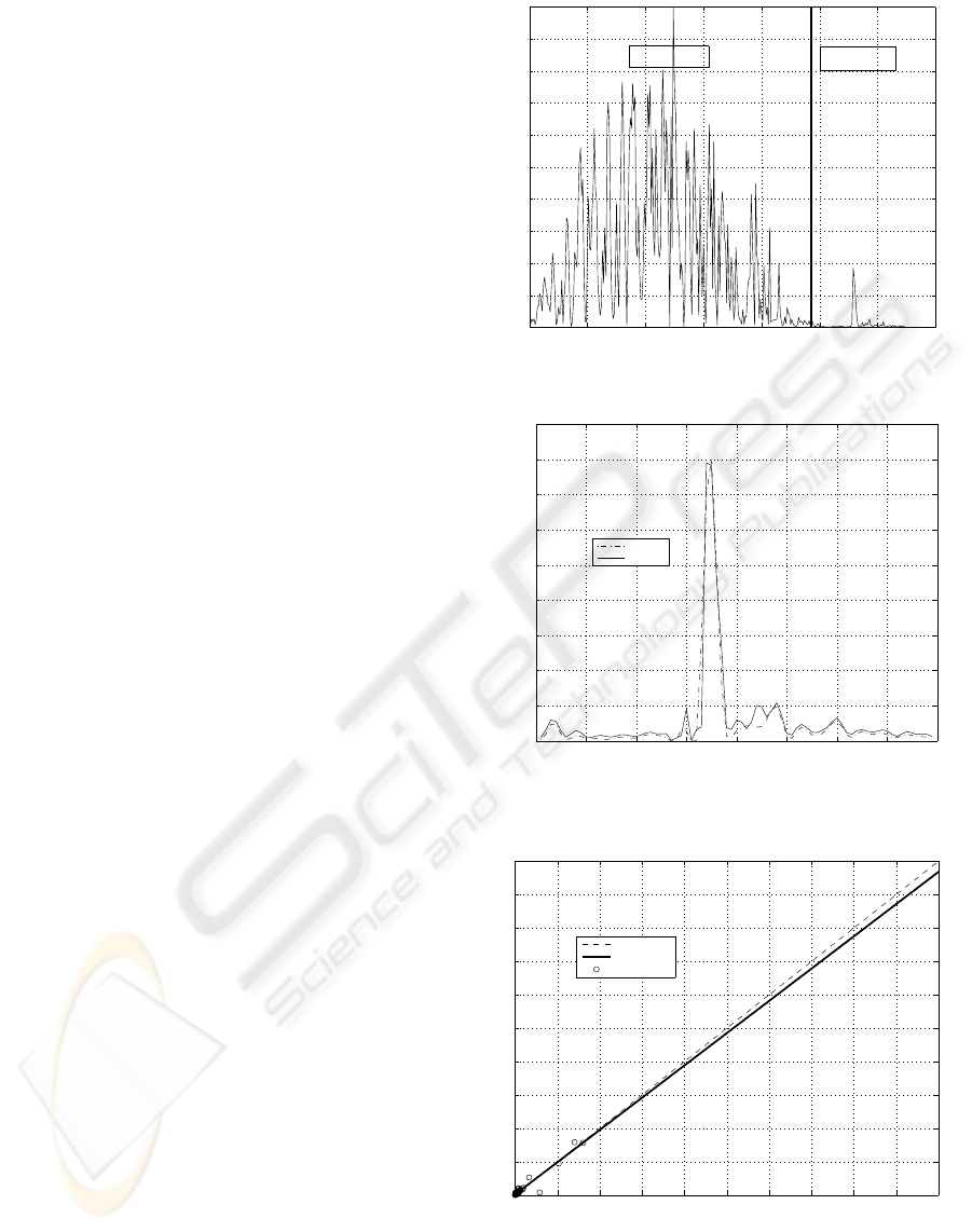
The observed monthly sardines catches data was con-
formed by historical data from January 1976 to De-
cember 2002, divided into two data subsets as shown
in Fig.1. In the first subset, 75% of historical data
was chosen for the training phase (weights estima-
tion), while the remaining 25% was used for the vali-
dation phase.
The forecasting process starts by applying the
wavelet denoising algorithm and normalization step
to the sardines catches data. Then, the hybrid learn-
ing algorithm is performed for training the (RBFNN)
model with normalize historical data. In the train-
ing phase, some important factors are selecting the
size of the input regression vector and the number
of hidden nodes. For selecting these parameters, a
trial-error scheme analysis was performed. In this
process, training the RBFNN model was achieved by
performing the learning algorithm with at most 3 it-
erations for a neural architecture (N
i
, N
h
, N
o
), where
N
i
= 8 represents the size of the input regression vec-
tor (number of input nodes), and N
h
= 4 and N
o
= 1
represent the number of hidden and output nodes, re-
spectively. In the evaluation phase, the accuracy of
the sardines catches forecasting is assessed by us-
ing the mean square error and determination coeffi-
cient. Fig.2 describes the performance evaluation of
the validation phase with testing data for the (8, 4, 1)-
forecasting model. From Fig.2 it can be observed that
the best forecasting model according to its parsimony
and precision is the architecture composed by 8 input
nodes, 4 hidden nonlinear nodes, and a linear output
node.
The regression between the observed and es-
timated sardines catches with the best forecasting
model based on RBFNN during the validation phase
is presented in Fig.3. Please note that the RBFNN
model shown that a 93% of the explained variance
was captured by the proposed forecasting model.
Moreover, from Fig.3 it is observed that the RBFNN
model significantly reduces determination coefficient,
since the hybrid algorithm avoids getting stuck into
local minima by combining least square method and
Levenberg Marquardt algorithm.
4 CONCLUSIONS
In this paper, one-step-ahead forecasting of monthly
sardines catches based on wavelet denoising and
RBFNN with hybrid algorithm has been pre-
sented. The forecasting model can predict the
future CPUE value based on previous values
0 50 100 150 200 250 300 350
0
0.1
0.2
0.3
0.4
0.5
0.6
0.7
0.8
0.9
1
CPUE
time (month)
TESTING= 25%
TRAINING= 75%
Figure 1: Monthly sardines catches data.
0 10 20 30 40 50 60 70 80
0
0.02
0.04
0.06
0.08
0.1
0.12
0.14
0.16
0.18
time (month)
CPUE
Real Data
Estimates
Figure 2: Observed sardines catches vs estimated sardines
catches with testing monthly data.
0 0.1 0.2 0.3 0.4 0.5 0.6 0.7 0.8 0.9 1
0
0.1
0.2
0.3
0.4
0.5
0.6
0.7
0.8
0.9
1
Ideal
Best Linear Fit
Data Points
Figure 3: Observed sardines catches.
s(t − 1),s(t − 2),..,s(t − 8) and the results found
show that proposed model gives a determination co-
efficient equal to 93% with a reduced parsimony and
ICSOFT 2008 - International Conference on Software and Data Technologies
310

fast convergence speed of the hybrid training algo-
rithm.
REFERENCES
Coifman, R. and Donoho, D. (1995). Translation-invariant
denoising, wavelets and statistics. In Springer Lecture
Notes in Statistics. vol. 103, pp. 125-150.
Donoho, D. (1995). De-noising by soft-thresholding. In
IEEE Trans. on Information theory. vol. 41, no. 3, pp.
613-627.
Hagan, M. and Menhaj, M. (1994). Training feed-forward
networks with marquardt algorithm. In IEEE Trans.
Neural networks. vol. 5, no. 6, pp. 1134-1139.
J. Gutierrez, C. Silva, E. Y. N. R. and Pulido, I. (2007).
Monthly catch forecasting of anchovy engraulis rin-
gens in the north area of chile: Nonlinear univariate
approach. In Fisher Research. vol. 86, pp. 188-200.
K. Hornik, M. S. and White, H. (1989). Multilayer feedfor-
ward networks are universal approximators. In Neural
network. vol. 2, no. 5, pp. 359-366.
Karayiannis, N. B. (1999). Reformulated radial basis neural
networks trained by gradient descent. In IEEE Trans.
Neural networks. vol. 10, no. 3, pp. 188-200.
Nason, G. and Silverman, B. (1995). Translation-invariant
denoising, wavelets and statistics. In Springer Lecture
Notes in Statistics. vol. 103, pp. 181-3000.
Pesquet, J.-C., K. H. and Carfantan, H. (1995). Time-
invariant orthonormal wavelet representations. In
IEEE Trans. on Signal Processing. vol. 44, no. 8, pp.
1964-1996.
Serre, D. (2002). Matrices: Theory and applications.
Springer Verlag, New York.
Stergiou, K. I. (1996). Prediction of the mullidae fishery in
the easterm mediterranean 24 months in advance. In
Fisher Research. vol.9, pp. 67-74.
Stergiou, K. I. and Christou, E. (1996). Prediction of
the mullidae fishery in the easterm mediterranean 24
months in advance. In Fisher. Research. vol. 25, pp.
105-138.
RBF NETWORK COMBINED WITH WAVELET DENOISING FOR SARDINE CATCHES FORECASTING
311
