REAL TIME CLUSTERING MODEL
J. Cheng, M. R. Sayeh
Department of Electrical and Computer Engineering
Southern Illinois University Carbondale, Carbondale, IL 62901, U.S.A.
M. R. Zargham
Department of Computer Science, Southern Illinois University Carbondale, Carbondale, IL 62901, U.S.A.
Keywords: ODE, Clustering, Vector quantization, Real time.
Abstract: This paper focuses on the development of a dynamic system model in unsupervised learning environment.
This adaptive dynamic system consists of a set of energy functions which create valleys for representing
clusters. Each valley represents a cluster of similar input patterns. The system includes a dynamic parameter
for the clustering vigilance so that the cluster size or the quantizing resolution can be adaptive to the density
of the input patterns. It also includes a factor for invoking competitive exclusion among the valleys; forcing
only one label to be assigned to each cluster. Through several examples of different pattern clusters, it is
shown that the model can successfully cluster these types of input patterns and form different sizes of
clusters according to the size of the input patterns.
1 INTRODUCTION
As stated in (Jain, 1988), "Cluster analysis is the
process of classifying objects into subsets that have
meaning in the context of a particular problem." In
other words, clustering is a process of grouping a set
of unlabeled data. As shown in Figure 1, in general,
clustering can be grouped into two types: non-
overlapping (exclusive) and overlapping
(nonexclusive). In non-overlaping, each object input
will be assigned to only one cluster whereas in
overlapping an object can be assigned to more than
one cluster. In this paper we only consider non-
overlapping clustering. Non-overlapping clustering
could lie either intrinsic or extrinsic. In the intrinsic
approach, also called unsupervised learning, a
proximity matrix is the only criteria used. (Proximity
matrix represents relationship between the objects; if
the objects are patterns such matrix could represent
the distance between the patterns). The extrinsic
approach, also called supervised learning, in
addition to proximity matrix, it also uses category
labels on the objects. To notice the difference
between these two approaches, let’s consider a set of
data representing
health condition of normal and
overweight children. Using intrinsic approach, we
can group these children based on these factors and
then try to determine whether overweight plays a
role in academic status. Taking an extrinsic
approach allow us to study the way of separating
normal and overweight children by considering their
health conditions.
We consider intrinsic approaches only. The
intrinsic methods can be
divided into five types:
hierarchical, partitional, grid-based,
artificial neural
networks, and evolutionary (Jain, 1988; MacQueen,
1967; Grossberg, 1976; and Kohonen, 1982).
Comparison of these clustering methods is hard
to do using simulation because of different
implementation of the methods and the data that is
used. It is also hard to do theoretically comparison
of them because they are almost impossible to model
mathematically (Jain, 1988). Furthermore, the
existing models impose architectural complexity
and/or time complexity which prevent them of
having real time response time. To overcome the
real time mathematical modeling problems, we have
proposed a new method which depends solely on
ordinary differential equations (ODE) (Cheng, 2006).
There is no need for IF/THEN logical statements.
Therefore it can be easily implemented on the
analog type devices to take advantage of high-speed
electronics or photonics technologies.
235
Cheng J., R. Sayeh M. and R. Zargham M. (2008).
REAL TIME CLUSTERING MODEL.
In Proceedings of the Tenth Inter national Conference on Enterprise Information Systems - AIDSS, pages 235-240
DOI: 10.5220/0001694002350240
Copyright
c
 SciTePress

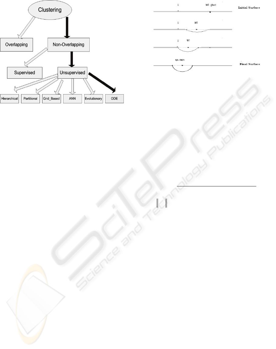
Figure 1: Different Clustering Methods.
The organization of this paper is as follows:
Section 2 describes the adaptive dynamical model
and devise an additional state for the dynamics of
vigilance parameter
λ
, which plays an important
role in our system; Section 3 illustrates the
performance of the proposed model on several
examples; Finally, Section 4 presents the conclusion.
2 THE CLUSTERING MODEL
The idea behind our model is to store input patterns
on the surface of an energy
function of a dynamic
system. The clusters are represented as valleys on
the surface of an energy function. To demonstrate
this concept, let’s consider an input U in one
dimensional space as shown in Figure 2. Also let W
be a representative of a cluster and is randomly
placed on the surface of the energy function as
shown in Figure 2 by a black dot. The energy
function is represented by the black line, and the
input U is denoted by a gray dot. As the dynamic
progresses, the W moves toward U and forms a
complete valley when it reaches to U. Similarly, in
cases where there are more than one input pattern,
the valleys are created for patterns that are close to
each other.
Figure 2: One-Dimensional Example of Process of
Clustering forming by our model.
Generally, considering an N dimensional space
for input patterns, the V energy function is
constructed to represent M valleys centered at
locations
(
)
T
Njjjj
wwwW ...,
,2,1
= , for
1=j
to M,
representing M clusters for
P
input patterns. The
V energy function is represented as
∑∑
==
⎥
⎦
⎤
⎢
⎣
⎡
−=
P
p
M
j
jp
xV
1
2
1
γ
Here,
2
||||1
1
jp
j
jp
WU
x
−+
=
λ
where
• is the Euclidean norm,
(
)
T
Njjjj
wwwW ...,
,2,1
= , for
1=j
to M, represent
center of valley j,
p
U
is the input pattern p,
M is the number of clusters, and
P is the number of input patterns.
W and U refer to vectors when N >1.
The constant
γ encourages a number of valleys
(clusters) to be formed and the factor
λ (vigilance
parameter) approximately reflects the radius of the
generated valley.
In order to invoke competitive exclusion among
the valleys, the following competitive C-energy
function is used
∑∑∑
== ≠
=
P
p
M
i
M
is
spip
xxC
11
This function guarantees only one of the valleys
encodes the patterns by achieving its minimal value.
Based on the above two functions, the total R-
energy function is constructed, which is the
summation of the V-energy function and C-energy
function.
ICEIS 2008 - International Conference on Enterprise Information Systems
236


∑∑∑∑∑
== ≠==
+
⎥
⎦
⎤
⎢
⎣
⎡
−=
P
p
M
i
M
is
spip
P
p
M
j
jp
xxxR
111
2
1
ργ
where ρ is a balancing factor.
The
j
λ
, j= 1,..,M, (vigilance parameter)
approximately reflects the radius of the generated
valley j. As
j
λ
gets smaller, valley j becomes wider.
The
),,...,1( Mjx
jp
=
which has a value between 0
and 1, represents the depth of valley j. As the
distance between
p
U
and
j
W
decreases, the value
of
jp
x
moves toward 1 indicating
j
W
as a cluster
for
p
U
. This model is a gradient dynamical system
with R; thus
)(*
4
2
11
ijip
p
j
M
q
M
qs
spqp
P
p
j
ij
wux
xx
w
R
−
⎥
⎦
⎤
⎢
⎣
⎡
+−−=
∂
∂
∑∑∑
=≠=
γλ
()
.
1
1
1
2
⎟
⎠
⎞
⎜
⎝
⎛
−+
=
∑
=
N
i
ijipj
jp
wu
x
λ

where
jp
x
is explicitly given as
Thus, the dynamics of the system can be expressed
as:
)(*
4
2
11
ijip
p
j
M
q
M
qs
spqp
P
p
j
ij
wux
xx
dt
dw
−
⎥
⎦
⎤
⎢
⎣
⎡
+−=
∑∑∑
=≠=
γλ
Now let’s consider system state for the vigilance
parameter λ so that the cluster size can be adaptive
to the size of the input patterns;
λ
adjust
is a
function which can be expressed as
∑∑
==
⎟
⎟
⎠
⎞
⎜
⎜
⎝
⎛
−=
M
j
P
p
jpj
initial
adjust
x
P
1
2
1
*
λ
γ
λ
λ
Here,
initial
λ
is the initial value of
λ
, usually
specified by the user.
The λ dynamics can be derived as
)(*
*
2
1
2
11 1
∑
∑∑ ∑
=
== =
−
⎥
⎦
⎤
⎢
⎣
⎡
−=
∂
∂
N
k
kjkp
p
j
P
p
M
j
P
q
jqj
initial
j
j
adjust
wux
x
P
λ
γ
λ
λ
λ
λ
3 CLUSTERING PERFORMANCE
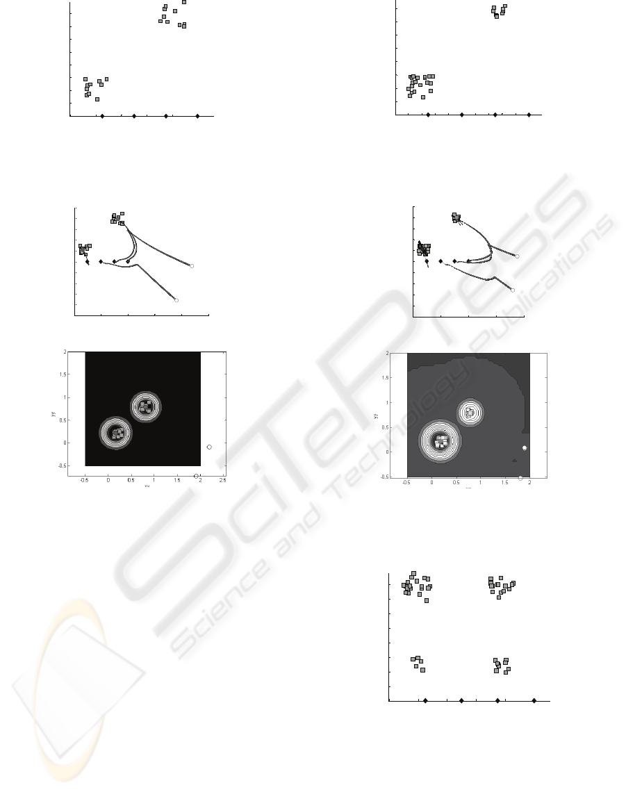
This section demonstrates simulation results of our
model on two sets and four sets of 2D input patterns
as shown in figures 3, 5, 7, and 10. In Figure 3, there
are two sets of input patterns where each one
includes10 inputs patterns. In Figure 5, there are two
sets of input patterns, one contains 20 and the other
contains10 inputs. In Figures 7 and 10, there are four
sets of input patterns, containing 5, 10, 15 and 20
inputs. Figures 3, 5, and 7 include 4 Ws while Figure
10 includes 6 Ws. Input patterns are denoted as
squares (gray color) and Ws represented as diamonds
(black color). The coordinate one and coordinate
two represent the first and second coordinates of
input patterns (U) and weights (W). Each set of
inputs are randomly generated having a value
between 0 and 1, while weights are placed at some
specific points. Figures 4(a), 6(a), 8(a), 9(a), and
11(a) demonstrate tracking paths and final positions
of the Ws in figures 3, 5, 7, 7 and 10, respectively.
The small circles represent the final position of Ws;
the ones with grey color represent the center of the
clusters formed by winner Ws; and the ones with
white color represent final position of Ws, which
cannot win the competition. Figures 4(b), 6(b), 8(b),
9(b), and 11(b) are the final contour images of the
energy function for each of these cases. The
surfaces of these images represent the V-energy
function in terms of different input values. Each
generated valley is represented by a set of nested
rings with different shades representing different
levels of valley’s depth (black represents the deepest
point and the dark gray represents the surface).
Figure 4 (a) demonstrates the set of obtained clusters
for initial λ equal to 20, and γ equal to 2. As can be
seen, two Ws win the competition to form clusters
for each set of inputs and the other two Ws move
away from the input patterns. As can be observed
from the contour image in Figure 4 (b), two valleys
are formed representing two different clusters.
REAL TIME CLUSTERING MODEL
237

0 0.2 0.4 0.6 0. 8 1
0
0.1
0.2
0.3
0.4
0.5
0.6
0.7
0.8
Dimension One (U & W)
Dimension Two (U & W)
Figure 3: Two clusters; there are 20 input patterns
(represented by squares) and 4
Ws (represented by the
diamonds) positioned at the bottom of the inputs.
0 0.5 1 1.5 2 2.5
-1
-0.8
-0.6
-0.4
-0.2
0
0.2
0.4
0.6
0.8
1
Dimension One (U & W)
Dimension Two (U & W)
(a) Moving path and final position of Ws.
(b) Contour representation.
Figure 4: Final positions of
Ws and contour representation
of the
V-energy function.
Figure 5 (a) demonstrates the set of obtained clusters
for initial λ equal to 20, and γ equal to 2. As can be
seen, two Ws win the competition and form clusters.
The other two Ws move away. In this simulation, λ
values from initial value 20 change to 15.7, 351.5,
260.2, and 29.3 for each of four Ws. Two winning
Ws have two different λ values 15.7 and 29.3 since
the two sets of input patterns have different size. The
other two runaway Ws have λ values as 351.5 and
260.2. The bigger set of input patterns corresponds
to smaller λ values (resulting bigger cluster), and the
smaller set of input patterns corresponds to bigger λ
values (resulting smaller cluster).
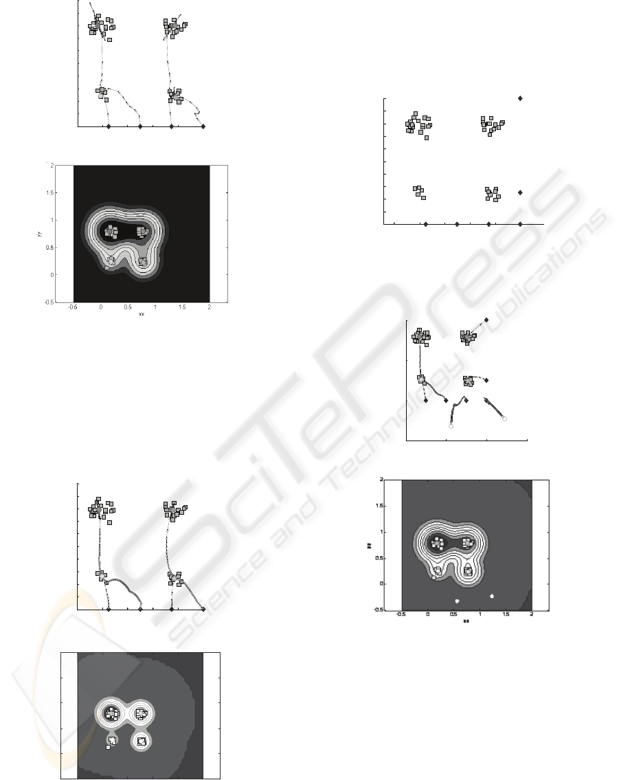
Figure 8 (a) demonstrates the set of obtained clusters
for initial λ equal to 20, and γ equal to 4. As can be
seen, four Ws form clusters for each set of inputs.
After simulation stops, λ values from initial value 20
change to 10.1, 11.9, 29.7, and 17.5 forming four
different size clusters.
0.1 0.2 0.3 0.4 0.5 0.6 0.7 0.8 0.9 1
0
0.1
0.2
0.3
0.4
0.5
0.6
0.7
0.8
Dimension One (U & W)
Dimension Two (U & W)
Figure 5: Two clusters; there are 30 input patterns
(represented by squares) and 4
Ws (represented by the
diamonds) positioned at the bottom.
0 0.5 1 1.5 2
-1
-0.8
-0.6
-0.4
-0.2
0
0.2
0.4
0.6
0.8
1
Dimens ion One (U & W )
Dimension Two (U & W)
(a) Moving path and final position of Ws.
(b) Contour representation.
Figure 6: Final positions of
Ws and contour representation
of the
V-energy function.
0 0.2 0.4 0.6 0.8 1
0
0.1
0.2
0.3
0.4
0.5
0.6
0.7
0.8
Dimension One (U & W)
Dimension Two (U & W)
Figure 7: Four clusters; there are 50 input patterns
(represented by squares) and 4
Ws (represented by the
diamonds) positioned at the bottom.
ICEIS 2008 - International Conference on Enterprise Information Systems
238


0 0.2 0.4 0.6 0.8 1
0
0.1
0.2
0.3
0.4
0.5
0.6
0.7
0.8
0.9
1
Dimens ion One (U & W )
Dimension Two (U & W)
(a) Moving path and final position of Ws.
(b) Contour representation.
Figure 8: Final positions of Ws and contour representation
of the
V-energy function.
Figure 9 (a) demonstrates the same experience as
Figure 8 (a) except in this case the initial value for λ
is set equal to 40. After simulation stops, λ values
from initial value 40 change to 24.2, 30.0, 84.4 and
43.8.
0 0.2 0.4 0.6 0.8 1
0
0.1
0.2
0.3
0.4
0.5
0.6
0.7
0.8
0.9
1
Dimension One (U & W)
Dimens ion Two (U & W)
(a) Moving path and final position of Ws
xx
yy
5328 (1772340310682865/2251799813685248-yy)
2
))-8532229875571793/72057594037927936/(1
+
-0.5 0 0.5 1 1.5 2
-0.5
0
0.5
1
1.5
2
(b) Contour representation
Figure 9: Final positions of
Ws and contour representation
of the
V-energy function.
Figure 11 (a) demonstrates the set of obtained
clusters for initial λ equal to 25, and γ equal to 4. As
can be seen, out of 6 Ws, four Ws win and form
clusters. After simulation stops, λ values for these
wining Ws become 13.3, 41.1, 15.9, and 23.4.
0 0.2 0.4 0.6 0.8 1
0
0.1
0.2
0.3
0.4
0.5
0.6
0.7
0.8
0.9
1
Dimension One (U & W)
Dimens ion Two (U & W)
Figure 10: Four clusters; there are 50 input patterns
(represented by squares) and 4
Ws (represented by the
diamonds) positioned at the right lower corner.
0 0.5 1 1.5
-0.5
0
0.5
1
Dimension One (U & W)
Dimension Two (U & W)
(a) Moving path and final position of Ws.
(b) Contour representation.
Figure 11: Final positions of
Ws and contour
representation of the
V-energy function.
4 CONCLUSIONS
The main purpose of this paper was the introduction
of a novel dynamical system for clustering which
has potential for real-time device realization. We
also devise an additional system state for the
vigilance parameter λ so that the cluster size or the
quantizing
resolution can be adaptive to the size of
REAL TIME CLUSTERING MODEL
239

the input patterns. This reduces the burden of re-
tuning the vigilance parameter for a given input
pattern set and it will also better represent the input
pattern space. These discussions are furthermore
visualized by simulation examples. As shown from
simulation results, our dynamic system can
successfully cluster different input patterns by
dynamically adjust λ values according to the size of
the input patterns in order to form different sizes of
clusters. In this system, self-organizing properties
can be implicitly coded within the system trajectory
structure using only ODE’s. These ODE’s can be
directly implemented in hardware through feed-back
networks by analog electronic or optical
implementation.
REFERENCES
Block, H.-H., 2002. Clustering Methods: From Classical
Models to New Approaches,
Statistics in Transition,
Vol. 5, No. 5, October 2002, pp. 725-758.
Grossberg, S. 1976. Adaptive pattern classification and
universal recoding, II: feedback, expectation, olfaction,
and illusions, Biological Cybernetics, 23, 187-202.
Jain, A. K., & Dubes, R. C. 1988.
Algorithms for
Clustering Data
. New Jersey: Prentice Hall,
Englewood Cliffs.
Kohonen, T. 1982. Self-organized formation of
topologically correct feature maps.
Biological
Cybernetics
, 43, 59-69.
MacQueen, J. B. 1967. Some methods for classification
and analysis of multivariate observations, Proceedings
of 5-th Berkeley Symposium on Mathematical
Statistics and Probability
, University of California
Press. Berkeley, 1:281-297.
Cheng, J., Sayeh, M.R., & Zargham, M.R. 2006. Neural
Net Based Models for Clustering.
International
Journal of Computational Intelligence Theory and
Practice, 1(2),
91-102.
ICEIS 2008 - International Conference on Enterprise Information Systems
240