
PRODUCTION CONFIGURATION OF PRODUCT FAMILIES
An Approach based on Petri Nets
Lianfeng Zhang, Brian Rodrigues
Department of Operations, University of Groningen, Landleven 5, Groningen, The Netherlands
Lee Kong Chian School of Business, Singapore Management University, Singapore
Jannes Slomp, Gerard J. C. Gaalman
Department of Operations, University of Groningen, Landleven 5, Groningen, The Netherlands
Keywords: Production configuration, Timed Petri nets, Colored Petri nets, Transition synchronization.
Abstract: Configuring production processes for product families has been acknowledged as an effective means of
dealing with product variety while maintaining production stability and efficiency. In an attempt to assist
practitioners to better understand and implement production configuration, we study the underlying logic for
configuring production processes for product families by means of dynamic modelling and visualization.
Accordingly, we develop a formalism of nested colored timed Petri nets (PNs) to model production
configuration. To cope with the modelling difficulties resulting from the fundamental issues in production
configuration, three types of nets, namely process nets, assembly nets and manufacturing nets, together with
a nested net system are defined by integrating the principles of colored PNs, timed PNs and nested PNs. An
industrial example of electronics products is used throughout the whole paper to demonstrates how the
proposed formalism is applied to specify production processes at differently levels of abstraction to achieve
production configuration.
1 INTRODUCTION
Facing a high variety of customized products often
required in small quantities and with short delivery
lead-times, manufacturing companies nowadays
strive to provide quickly diverse products at low
costs so as to survive the intense global competition.
It has been recognized that the key for companies to
achieving efficiency in the resulting high variety
production lies in an ability to maintain it to be as
stable as possible (Martinez et al., 2000). In this
respect, process configuration contributes to
obtaining manufacturing stability by generating
similar manufacturing processes for parts
(Schierholt, 2001). It, de facto, is an alternative
computer-aided process planning and thus does not
lend itself to achieve efficiency in producing product
families, where both assemblies and parts are
involved. In response to the limited research in
product family production , production configuration
has been proposed for companies to produce product
variety while achieving mass production efficiency
(Zhang, 2007). The rationale is to plan and utilize
similar, yet optimal, production processes as these
existing on shop floors to fulfil customized products.
Production configuration entails a conceptual
structure and overall logical organization of
producing a family of individualized products. It
provides a generic umbrella to capture and utilize
commonality, within which each new product
fulfilment is instantiated and extended, and thereby
anchoring planning to a common structure of a
product family (Zhang et al., 2007). Underpinned by
the common structure, production configuration
involves such common elements as operations and
processes concepts for parts and assemblies,
operations and their precedence, and manufacturing
resources. Also involved are diverse optional
process elements in accordance with optional parts
and assemblies. Production configuration entails a
process of 1) selecting proper elements for given
products; 2) subsequently arranging the selected
elements into production processes; and 3) finally
evaluating the configured multiple alternatives to
5
Zhang L., Rodrigues B., Slomp J. and J. C. Gaalman G. (2008).
PRODUCTION CONFIGURATION OF PRODUCT FAMILIES - An Approach based on Petri Nets.
In Proceedings of the Tenth International Conference on Enterprise Information Systems - ISAS, pages 5-11
DOI: 10.5220/0001669400050011
Copyright
c
SciTePress

determine appropriate ones. In such selection,
arrangement and evaluation processes, a number of
configuration rules, i.e., constraints or restrictions
imposed by manufacturing capabilities, capacity
limits, desired objectives that measure productivity
and efficiency, etc. must be satisfied. Consequently,
decision making in production configuration is
deemed to be very complex.
With an attempt to assist practitioners to better
understand and implement production configuration,
in this study, we tackle the underlying logic for
configuring production processes for product
families. In view of the potential of dynamic
modelling and visualization in shedding light on
process logic, we propose to model production
configuration graphically. In relation to fundamental
issues in production configuration (Zhang, 2007),
the resulting difficulties in modelling production
configuration have been identified. They include 1)
handling a high product and process variety; 2)
accommodating many process variations resulting
from design changes; 3) dealing with configuration
at different abstraction levels; 4) satisfying a number
of constraints/restrictions describing, for example,
the connections between product and process
elements; and 5) selecting process elements/
processes from multiple alternatives.
Owing to their executability, graphical
representation and mathematic support, Petri nets
(PNs) have been well recognized as a powerful
modelling, simulation and evaluation tool for
complex flows and processes (Peterson, 1981). A
number of extensions have been made to classic PNs
in order to satisfy different modelling requirements.
Among all, colored PNs (CPNs; Jensen, 1995),
timed PNs (TPNs; Ramachandani, 1974) and nested
PNs (NPNs; Lomazova, 2000) are of particular
interest in this study. CPNs are able to provide a
concise, flexible and manageable representation of
large systems by attaching a variety of colors to
tokens. By including timing, TPNs can capture
systems physical behaviours through assuming
specific durations for various activities. By
considering PNs as tokens, NPNs is expected to
model large and complex system through refinement
and abstraction.
In this paper, we apply PN techniques to model
production configuration by taking into account the
difficulties imposed by the fundamental issues.
Accordingly, a formalism of NCTPNs (nested
colored timed PNs) has been developed by
integrating the basic principles of CPNs, TPNs and
NPNs. Product/process variety and configuration
constraints are handled by attaching various data
describing product items and process elements to
tokens, resulting colored tokens. A reconfiguration
mechanism is incorporated into the modelling
formalism to cope with process variations. Timing is
introduced to facilitate the selection of proper
machines, operations and processes. Moreover, a
multilevel net system is further developed based on
net nesting in NPNs to tackle explicitly the
granularity issue in production configuration.
The next section introduces an industrial
example of vibration motors for mobile phones,
which is used throughout the rest of this paper to
demonstrate the proposed formalism and the
modelling of production configuration.
2 INDUSTRIAL EXAMPLE
The industrial example adopted is the production of
vibration motors for mobile phones. The increasing
variations in mobile phones design lead to large
numbers of customized vibration motors to be
produced. Together with other factors, e.g., short
delivery lead times, the high variety of vibration
motors complicate the planning of their production
processes.
Modelling production configuration of a
vibration motor family using the proposed NCTPNs
is presented in this study. Figure 1 shows the
common product structure of the motor family. This
motor family assumes several part types, as shown
in the figure. According to the design requirements,
individual motors may not contain a specific variant
from each part family. In other words, not all part
types are assumed by each individual motor variant.
While the company produces all assembly families
and final motors, among all they manufacture
several part families, e.g., Ba family, Bb family, Tl
family.
VM
Rh
BA
AA
FA
CA
St Mt
Fm
Cl
Tp
Ct
Wt
Ba
Bb
Tl
: Part; : Assembly
FA: Frameassy; BA: Bracketassy; Rh: Rubber holder; Wt: Weight
VM: Vibration motor; AA: Armatureassy
CA: Coilassy; St: Shaft; Fm: Frame; Mt: Magnet; Ba: Bracket a
Bb: Bracket b; Tl: Terminal; Ct: Commutator; Cl: Coil; Tp: Tape
VM
Rh
BA
AA
FA
CA
St Mt
Fm
Cl
Tp
Ct
Wt
Ba
Bb
Tl
: Part; : Assembly
FA: Frameassy; BA: Bracketassy; Rh: Rubber holder; Wt: Weight
VM: Vibration motor; AA: Armatureassy
CA: Coilassy; St: Shaft; Fm: Frame; Mt: Magnet; Ba: Bracket a
Bb: Bracket b; Tl: Terminal; Ct: Commutator; Cl: Coil; Tp: Tape
Figure 1: The common product structure.
ICEIS 2008 - International Conference on Enterprise Information Systems
6

3 NET DEFINITIONS
Production configuration entails a process of
configuring a complete production process for a
product along with the product hierarchy, i.e., at
different levels of abstraction. Being located at the
highest level, the more abstract production process
involving the product’s immediate child items only
is configured first. Subsequently, the assembly
processes and/or manufacturing processes for
producing these immediate child items are
configured at the second level, and so on. The
manufacturing processes for parts at the lowest level
of each branch of the hierarchy are configured at
last. Bearing in mind the similarities embedded in
processes of any type, e.g., adoption of buffers and
alternative machines, involvement of WIPs, we
define a basic PN structure first, which reflects the
generalized common process elements that are
assumed by different types of nets defined in the
proposed formalism.
3.1 Basic Net Structure
Definition 1: A basic PN structure is a directed
bipartite graph
()
h,A,T,PG = , where
CRRIB
P
P
P
P
P
∪∪∪= is a finite set of places
with 4 disjoint subsets:
B
P
representing buffers (be it
for raw materials, parts, assemblies, or final
products),
I
P
items ready to be processed (be it a
raw material, part, assembly, or WIP),
R
P
machines,
and
CR
P
the conceptual machines for alternative
machines that can complete same tasks using
different operations;
φ
=∩∪∪= TP,TTTT
TRL
is a finite set of
transitions with 3 disjoint subsets:
L
T
denoting a set
of logical transitions,
R
T
a set of reconfigurable
transitions, and
T
T
a set of timed transitions;
PTTPA ×∪×⊆
is a finite set of arcs that
connect places/transitions to transitions/places; and
φ
=∩×⊆ Ah,TPh
RCR
is a finite set of inhibitor
arcs that connect a conceptual machine place to a
reconfigurable transition.
()
RCR
Tt,Pp,1t,ph ∈∈∀=
indicates that there is a token in the conceptual
machine place; and the associated reconfigurable
transition is disabled and cannot fire. When
()
,0t,ph = no token resides in the conceptual
machine place; and the associated reconfigurable
transition can fire if it is enabled.
Attempting to capture and model multiple
alternative machines in relation to same tasks,
CR
P
is defined in the formalism to represent the
corresponding conceptual machines in addition to
R
P
, which is defined to denote specific machines. In
conjunction with
CR
P
, h and
R
T
are introduced to
model the situations, where multiple machines can
perform same tasks and only one is used eventually.
The firing of
R
T
leads to the reconfiguration of
proper machines. In this way,
CR
P
,
R
T
and h can
address process variations in system models without
rebuilding new ones when machines are added
and/or removed.
L
T
is defined to capture the logic of the system
running. Their firing indicates the satisfaction of
preconditions of operations, for example, the
presence of material items and machines to be used.
T
T
is defined to represent operations, which take
certain time durations to complete. Thus, the firing
of timed transitions incurs time delays. Both logic
and reconfigurable transitions are untimed. Their
firing is instantaneous and takes 0 time delay.
Figure 2 shows a basic PN structure and the
corresponding graphical formalism. Based on the
basic PN structure, 3 types of PNs, namely
manufacturing nets (
MNets ), assembly nets ( ANets )
and a process net (
PNet ) are defined to address the
granularity issue in production configuration. These
nets are defined as a type with a marking, with each
type following the basic PN structure and includes
additional information.
: Place;
: Logical transition
: Arc;
: Reconfigurable transition
: Inhibitor arcs;
: Timed transition;
1
p
2
p
1
t
2
t
4
t
3
p
6
p
5
p
4
p
3
t
: Place;
: Logical transition
: Arc;
: Reconfigurable transition
: Inhibitor arcs;
: Timed transition;
1
p
2
p
1
t
2
t
4
t
3
p
6
p
5
p
4
p
3
t
Figure 2: A basic PN structure.
3.2 Manufacturing Net (MNet)
Definition 2: A manufacturing net is defined as a
tuple
(
)
μ
,ToMMNet
=
, where
MNet is a manufacturing net representing the
processes of manufacturing a part family;
(
)
τΕβαΣ
,,,,,GToM
M
= is a manufacturing type
with
−
G is the basic PN structure;
−
M
Σ
is a finite set of color sets or token types;
−
M
MP
Σ
α
6: is a color assignment function that
maps a place,
p
, to a set of colors,
()
p
α
;
PRODUCTION CONFIGURATION OF PRODUCT FAMILIES - An Approach based on Petri Nets
7
−
(
)
{
}
(
)
εΣΣβ
∪×:
MM
T 6 is a color assignment
function that maps a transition,
t , to a set of color
pairs,
()
t
β
such that each pair declares the transition,
t , must be synchronized externally with transitions
of the net where this manufacturing net resides,
except if the pair is
(
)
εΣ
,
M
, indicating no
synchronization is required;
−
()
τΣΕ
ΣΣΣ
+→∧∨∪∨×:
MMM
M@MMA
M
6 is
an arc expression function that defines the timed and
untimed arc expressions for arcs with respect to
transition colors;
∧
∨ / denote Exclusive OR
(XOR)/AND relationships; and
→ represents “if–
then”;
−
+
ℜ∈
τ
is a set of positive real numbers
representing time delays;
()
Pp,MP
p
∈∀:
α
μ
6 is a marking function
specifying the distribution of colored tokens in all
places of an
MNet .
While tokens in idle machine places are defined
to represent machines, tokens in busy machine
places are defined according to the items to be
produced. When there is a token residing in the
conceptual machine place, the conceptual machine is
instantiated to the specific machine represented by
the token. Cycle times are used to accommodate
selection of proper processes elements. Thus, time
delays,
τ
, are defined in the formalism to represent
operations cycle times.
To cope with the difficulties in modelling diverse
cycle times, an arc expression function,
Ε
, is
introduced in the formalism. It defines both timed
arc expressions and untimed arc expressions. A
timed arc expression is a set of antecedent-
consequent statements with XOR relationships. It
specifies input items, machines to be used, output
items and the cycle times to be incurred. Untimed
arc expressions are defined to specify 1) the input
tokens for firing any transitions; and 2) output
tokens after firing timed and reconfigurable
transitions.
6
p
1
p
9
p
1
t
7
t
321
AAAAAA ∨∨
32
1
ABAB
AB
∨
∨
10
p
()
()
()
()
()
()
()
12@ABmBAAA
9@ABmBAAA
13@ABmBAAA
11@ABmBAAA
15@ABmBAAA
12@ABmBAAA
10@ABmBAAA
3333
3233
2322
2122
1311
1211
1111
+→∧∧
∨+→∧∧
∨+→∧∧
∨+→∧∧
∨+→∧∧
∨+→∧∧
∨+→∧∧
2
p
4
p
3
p
2
t
3
t
4
t
8
p
3
2
1
m
m
m
∨
∨
6
t
5
p
() ( )( )( ){}
3322112
BA,BA,BA,BA,BA,BAt =
β
() ( )( )( ){}
;AA,AA,AA,AA,AA,AAt
3322111
=
β
() () ( )( )( ){}
;AB,,AB,,AB,tt
32173
εεεββ
==
9
t
16
p
12
t
17
p
11
p
8
t
21
FAFA ∨
12
p
3
m
2
m
1
m
32
1
MBMB
MB
∨
∨
()
()
()
()
7.11@MBmFAAB
6.10@MBmFAAB
2.14@MBmFAAB
8.12@MBmFAAB
3423
2522
1511
1411
+→∧∧
∨+→∧∧
∨+→∧∧
∨+→∧∧
()
(
)
{
}
14
m,t
εβ
=
() ( ){}
;m,t
25
εβ
=
()()()()(){}
;MB,,MB,,MB,tt
321129
εεεββ
==
() ( )( ){}
;FA,FA,FA,FAt
22118
=
β
10
t
14
p
15
p
5
4
m
m ∨
4
m
5
m
11
t
13
p
4
m
5
m
4
m
5
m
18
p
()
()
()
8.7@VMmRhWtMB
7.6@VMmRhMB
2.6@VMmWtMB
16111
3623
2622
+→∧∧∧
∨+→∧∧
∨
+
→
∧
∧
5
t
7
p
6
m
19
p
6
m
20
p
21
p
13
t
14
t
321
AAAAAA ∨∨
321
BABABA ∨∨
321
BABABA ∨∨
32
1
AAAA
AA
∨
∨
32
1
BABA
BA
∨
∨
3
m
2
m
1
m
3
m
2
m
1
m
32
1
ABAB
AB
∨
∨
32
1
ABAB
AB
∨
∨
21
FAFA ∨
2
1
FA
FA ∨
32
1
VMVM
VM
∨
∨
32
1
VMVM
VM
∨
∨
(
)
22
11
RhWt
RhWt
∨
∨∧
32
1
MBMB
MB
∨
∨
32
1
MBMB
MB
∨
∨
() ( ){}
;m,t
36
εβ
=
(
)( ){}
;m,t
410
εβ
=
() ( ){}
;m,t
511
εβ
=
() () ( )
(
)
(
){}
3211413
VM,,VM,,VM,tt
εεεββ
==
6
p
1
p
9
p
1
t
7
t
321
AAAAAA ∨∨
32
1
ABAB
AB
∨
∨
10
p
()
()
()
()
()
()
()
12@ABmBAAA
9@ABmBAAA
13@ABmBAAA
11@ABmBAAA
15@ABmBAAA
12@ABmBAAA
10@ABmBAAA
3333
3233
2322
2122
1311
1211
1111
+→∧∧
∨+→∧∧
∨+→∧∧
∨+→∧∧
∨+→∧∧
∨+→∧∧
∨+→∧∧
2
p
4
p
3
p
2
t
3
t
4
t
8
p
3
2
1
m
m
m
∨
∨
6
t
5
p
() ( )( )( ){}
3322112
BA,BA,BA,BA,BA,BAt =
β
() ( )( )( ){}
;AA,AA,AA,AA,AA,AAt
3322111
=
β
() () ( )( )( ){}
;AB,,AB,,AB,tt
32173
εεεββ
==
9
t
16
p
12
t
17
p
11
p
8
t
21
FAFA ∨
12
p
3
m
2
m
1
m
32
1
MBMB
MB
∨
∨
()
()
()
()
7.11@MBmFAAB
6.10@MBmFAAB
2.14@MBmFAAB
8.12@MBmFAAB
3423
2522
1511
1411
+→∧∧
∨+→∧∧
∨+→∧∧
∨+→∧∧
()
(
)
{
}
14
m,t
εβ
=
() ( ){}
;m,t
25
εβ
=
()()()()(){}
;MB,,MB,,MB,tt
321129
εεεββ
==
() ( )( ){}
;FA,FA,FA,FAt
22118
=
β
10
t
14
p
15
p
5
4
m
m
∨
4
m
5
m
11
t
13
p
4
m
5
m
4
m
5
m
18
p
()
()
()
8.7@VMmRhWtMB
7.6@VMmRhMB
2.6@VMmWtMB
16111
3623
2622
+→∧∧∧
∨+→∧∧
∨
+
→
∧
∧
5
t
7
p
6
m
19
p
6
m
20
p
21
p
13
t
14
t
321
AAAAAA ∨∨
321
BABABA ∨∨
321
BABABA ∨∨
32
1
AAAA
AA
∨
∨
32
1
BABA
BA
∨
∨
3
m
2
m
1
m
3
m
2
m
1
m
32
1
ABAB
AB
∨
∨
32
1
ABAB
AB
∨
∨
21
FAFA ∨
2
1
FA
FA ∨
32
1
VMVM
VM
∨
∨
32
1
VMVM
VM
∨
∨
(
)
22
11
RhWt
RhWt
∨
∨∧
32
1
MBMB
MB
∨
∨
32
1
MBMB
MB
∨
∨
() ( ){}
;m,t
36
εβ
=
(
)( ){}
;m,t
410
εβ
=
() ( ){}
;m,t
511
εβ
=
() () ( )
(
)
(
){}
3211413
VM,,VM,,VM,tt
εεεββ
==
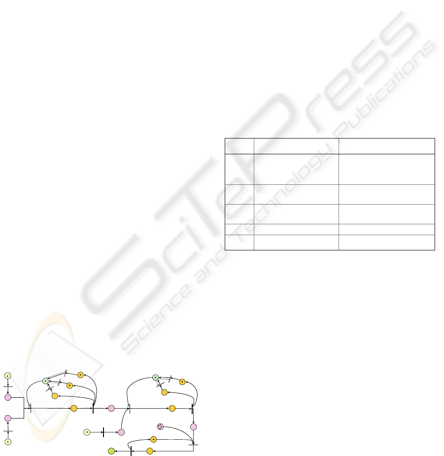
Figure 3: The PNet of the motor family.
By following the common routing of the motor
family, the
PNet is constructed, as shown in Figure
3. In the
PNet , the involved items include AAs,
FAs, BAs, ABs (abassies; WIPs formed by AAs and
BAs), MBs (mainbodies; WIPs formed by ABs and
FAs) and VMs. The places, represented system
elements and contained colored tokens/lower level
nets are listed in Table 1 (not exhaust due to place
constraints). The color pairs assigned to each
transaction are shown in the figure. For illustrative
simplicity, the colored tokens in relation to 3 motor
variants (
21
VM,VM and
3
VM ) are given in Figure 3
and Table 1, and in the following figures and tables
as well. Take the timed arc expression of arc
(
)
2013
p,t as an example. It shows that
1
VM assumes
both Wt and Rh;
2
VM contains a Wt; and
3
VM
includes an Rh. Also shown are the machines used
and the corresponding cycle times.
Table 1: The places, represented system elements and
colored tokens/nets.
Places System Elements Nets/Colored Tokens
11/4/1
p
Input buffers for
AAs/Bas /FAs
ANets for producing
assembly
families AA/BA/FA
2
p
AAs are ready to be
processed
(){ }
3212
AA,AA,AAp =
α
3
p
BAs are ready to be
processed
(){ }
3212
BA,BA,BAp =
α
… … …
21
p
A buffer for final motors
(){ }
32121
VM,VM,VMp =
α
3.3 Assembly Net (ANet)
Definition 3: An assembly net is defined as a tuple
(
)
μ
,ToAANet =
, where
ANet is an assembly net representing the
processes of producing a family of assembly
variants;
(
)
τΕβαΣ
,,,,,SoTma,GToA
A
= is an assembly
type with
−
G is the basic PN structure;
−
SoTma is a set of manufacturing types and
assembly types;
−
A
Σ
is a finite set of color sets or token types;
−
A
MSoTmaP
Σ
α
∪: 6 is an assignment function
that maps a place,
p
, to manufacturing or assembly
types or a set of colors;
−
{
}
(
)
(
)
{}
(
)
εΣΣεΣβ
∪××∪:
AAA
T 6 is an
assignment function that maps a transition,
t , to a set
of color triples,
(
)
t
β
, such that each triple declares
ICEIS 2008 - International Conference on Enterprise Information Systems
8
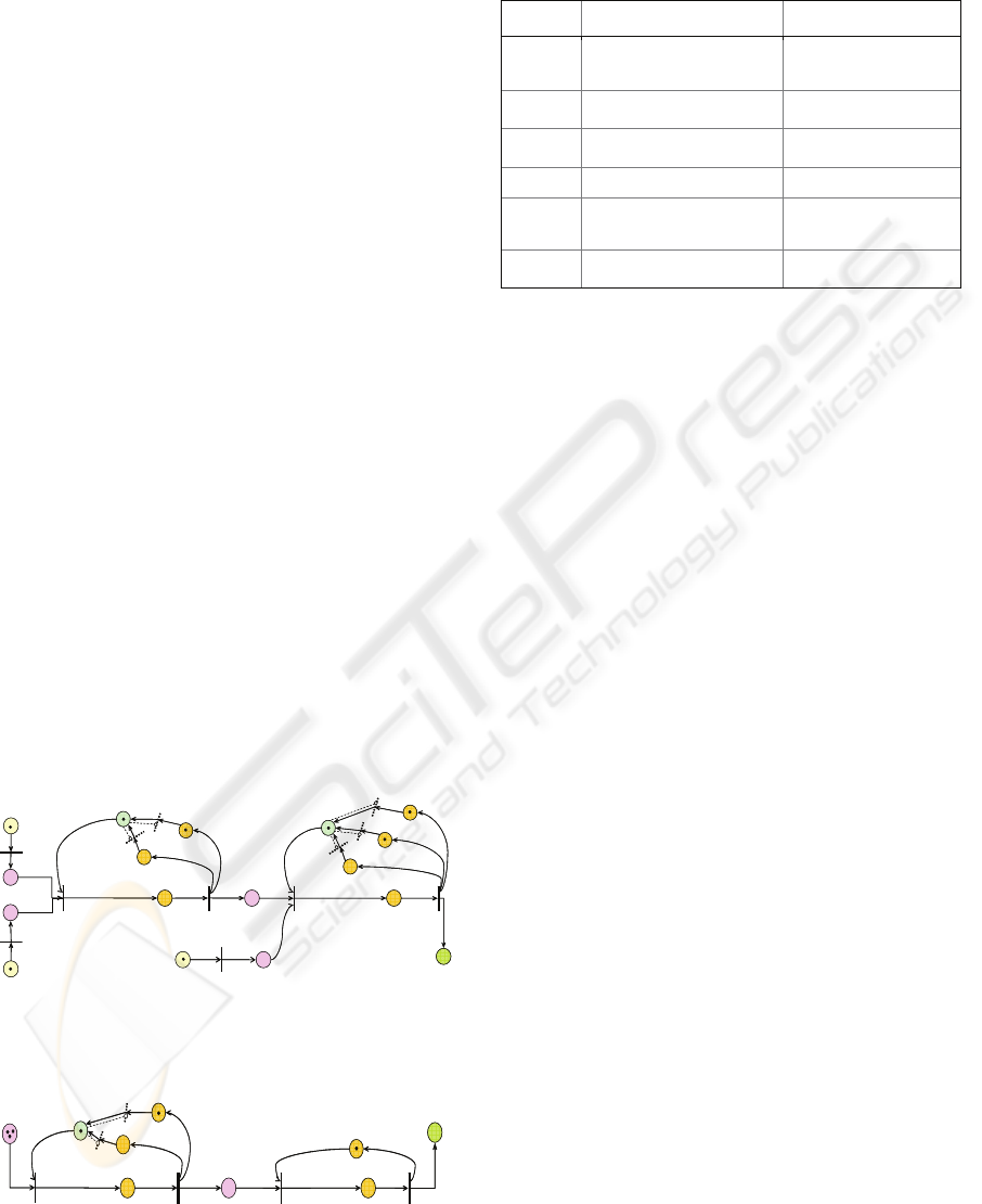
the transition,
t , must be synchronized 1) internally
with transitions of the nested net; and 2) externally
with transitions of the host net where this assembly
net is contained, except if the triple is
(
)
εΣε
,,
A
;
−
()
τΣΕ
ΣΣΣ
+→∧∨∪∨×:
AAA
M@MMA
A
6 is
an arc expression function that defines the timed and
untimed arc expressions for arcs with respect to
transition colors; and
−
+
ℜ∈
τ
is a set of positive real numbers
representing time delays;
()
Pp,MP
p
∈∀:
α
μ
6 is a marking function
specifying the distribution of colored tokens,
manufacturing and assembly nets in all places of an
ANet .
Unlike raw buffer places in an
MNet , buffer
places in an
ANet are defined for the immediate child
items of assemblies. Tokens in such
part/subassembly buffers are
MNets / ANets of child
items. The assignment function,
α
, specifies the
allocation of such
MNets / ANets to buffer places and
colored tokens to other places.
Same as specifying the
PNet , four
ANets
have
been constructed for 4 assembly families of the
motor family in Figure 1. Figure 4 shows the
ANet
of BA family. The color triples assigned to each
transition are also shown. According to these
colored triples, transitions of this
ANet fires
autonomously, or simultaneously with either the
transitions of the nested nets residing in places
2522
p,p
and
31
p
or the transitions of the PNet in
Figure 3. Table 2 lists the set of places, represented
system elements and colored tokens/
MNets .
22
p
29
p
15
t
20
t
321
BaBaBa ∨∨
32
1
BabBab
Bab
∨
∨
30
p
()
()
()
()
()
()
3.6@BabmTlBbBa
3.5@BabmTlBbBa
1.6@BabmTlBbBa
6.5@BabmTlBbBa
9.4@BabmBbBa
3.4@BabmBbBa
38233
37233
28122
27122
1811
1711
+→∧∧∧
∨+→∧∧∧
∨+→∧∧∧
∨+→∧∧∧
∨+→∧∧
∨+→∧∧
23
p
25
p
24
p
16
t
17
t
23
t
34
p
36
p
11
10
9
m
m
m
∨
∨
25
t
33
p
() ( )( )( ){}
;,Ba,Ba,,Ba,Ba,,Ba,Bat
33221115
εεεβ
=
22
t
37
p
26
t
38
p
31
p
21
t
21
TlTl ∨
32
p
10
m
()
()
()
()
()
()
()
2.4@BAmTlBab
0.3@BAmTlBab
5.3@BAmTlBab
9.3@BAmTlBab
8.2@BAmTlBab
2.3@BAmTlBab
0@BABab
31123
31023
3923
21112
21012
2912
11
+→∧∧
∨+→∧∧
∨+→∧∧
∨+→∧∧
∨+→∧∧
∨+→∧∧
∨+→
18
t
27
p
28
p
8
7
m
m ∨
7
m
19
t
26
p
8
m
24
t
35
p
321
BbBbBb ∨∨
11
m
9
m
32
1
BABA
BA
∨
∨
() ( ){}
;,m,t
819
εεβ
=
321
BaBaBa ∨∨
321
BbBbBb ∨∨
32
1
BaBa
Ba
∨
∨
32
1
BbBb
Bb
∨
∨
7
m
8
m
7
m
8
m
10
m
11
m
9
m
10
m
11
m
9
m
32
1
BabBab
Bab
∨
∨
32
1
BabBab
Bab
∨
∨
21
TlTl ∨
2
1
Tl
Tl ∨
32
1
BABA
BA
∨
∨
() ( )( )( ){}
;,Bb,Bb,,Bb,Bb,,Bb,Bbt
33221116
εεεβ
=
() () ( )
(
)
(
){}
εεεεεεββ
,Bab,,,Bab,,,Bab,tt
3212017
==
() ( )( )( ){}
;,Tl,Tl,,Tl,Tl,,Tl,Tlt
33221121
εεεβ
=
()()()(){}
;,BA,,,BA,,,BA,t
32122
εεεεεεβ
=
(
)
(
)
{
}
εεβ
,m,t
923
=
() ( )( )
(
){}
23221126
BA,BA,,BA,BA,,BA,BA,t
εεεβ
=
() ( ){}
;,m,t
718
εεβ
=
() ( ){}
;,m,t
1024
εεβ
=
() ( ){}
;,m,t
1125
εεβ
=
22
p
29
p
15
t
20
t
321
BaBaBa ∨∨
32
1
BabBab
Bab
∨
∨
30
p
()
()
()
()
()
()
3.6@BabmTlBbBa
3.5@BabmTlBbBa
1.6@BabmTlBbBa
6.5@BabmTlBbBa
9.4@BabmBbBa
3.4@BabmBbBa
38233
37233
28122
27122
1811
1711
+→∧∧∧
∨+→∧∧∧
∨+→∧∧∧
∨+→∧∧∧
∨+→∧∧
∨+→∧∧
23
p
25
p
24
p
16
t
17
t
23
t
34
p
36
p
11
10
9
m
m
m
∨
∨
25
t
33
p
() ( )( )( ){}
;,Ba,Ba,,Ba,Ba,,Ba,Bat
33221115
εεεβ
=
22
t
37
p
26
t
38
p
31
p
21
t
21
TlTl ∨
32
p
10
m
()
()
()
()
()
()
()
2.4@BAmTlBab
0.3@BAmTlBab
5.3@BAmTlBab
9.3@BAmTlBab
8.2@BAmTlBab
2.3@BAmTlBab
0@BABab
31123
31023
3923
21112
21012
2912
11
+→∧∧
∨+→∧∧
∨+→∧∧
∨+→∧∧
∨+→∧∧
∨+→∧∧
∨+→
18
t
27
p
28
p
8
7
m
m ∨
7
m
19
t
26
p
8
m
24
t
35
p
321
BbBbBb ∨∨
11
m
9
m
32
1
BABA
BA
∨
∨
() ( ){}
;,m,t
819
εεβ
=
321
BaBaBa ∨∨
321
BbBbBb ∨∨
32
1
BaBa
Ba
∨
∨
32
1
BbBb
Bb
∨
∨
7
m
8
m
7
m
8
m
10
m
11
m
9
m
10
m
11
m
9
m
32
1
BabBab
Bab
∨
∨
32
1
BabBab
Bab
∨
∨
21
TlTl ∨
2
1
Tl
Tl ∨
32
1
BABA
BA
∨
∨
() ( )( )( ){}
;,Bb,Bb,,Bb,Bb,,Bb,Bbt
33221116
εεεβ
=
() () ( )
(
)
(
){}
εεεεεεββ
,Bab,,,Bab,,,Bab,tt
3212017
==
() ( )( )( ){}
;,Tl,Tl,,Tl,Tl,,Tl,Tlt
33221121
εεεβ
=
()()()(){}
;,BA,,,BA,,,BA,t
32122
εεεεεεβ
=
(
)
(
)
{
}
εεβ
,m,t
923
=
() ( )( )
(
){}
23221126
BA,BA,,BA,BA,,BA,BA,t
εεεβ
=
() ( ){}
;,m,t
718
εεβ
=
() ( ){}
;,m,t
1024
εεβ
=
() ( ){}
;,m,t
1125
εεβ
=
Figure 4: The ANet of the bracketassy family.
43
p
30
t
44
p
(
)
()
()
()
()
()
8.4@2.Bam1.Ba
4.4@2.Bam1.Ba
5.4@2.Bam1.Ba
7.3@2.Bam1.Ba
9.5@2.Bam1.Ba
3.5@2.Bam1.Ba
3133
3123
2132
2122
1131
1121
+→∧
∨+→∧
∨+→∧
∨+→∧
∨+→∧
∨+→∧
27
t
45
p
()()()()(){}
;,2.Ba,,2.Ba,,2.Batt
3213027
εεεββ
==
31
t
46
p
32
t
(
)
(
)
{
}
;,mt
1228
εβ
=
28
t
41
p
42
p
13
12
m
m ∨
12
m
29
t
40
p
13
m
14
m
(
)
(
)
{
}
;,mt
1329
εβ
=
1.Ba1.Ba
1.Ba
32
1
∨
∨
2.Ba2.Ba
2.Ba
32
1
∨
∨
2.Ba2.Ba
2.Ba
32
1
∨
∨
2.Ba2.Ba
2.Ba
32
1
∨
∨
(
)
()
()
5.1@Bam2.Ba
7.1@Bam2.Ba
1.1@Bam2.Ba
3143
2142
1141
+→∧
∨+→∧
∨+→∧
32
1
BaBa
Ba
∨
∨
32
1
BaBa
Ba
∨
∨
14
m
12
m
13
m
12
m
13
m
() ( )( )( ){}
;,Ba,,Ba,,Bat
32131
εεεβ
=
() ( )
(
)
(
){}
33221132
Ba,Ba,Ba,Ba,Ba,Bat =
β
39
p
47
p
43
p
30
t
44
p
(
)
()
()
()
()
()
8.4@2.Bam1.Ba
4.4@2.Bam1.Ba
5.4@2.Bam1.Ba
7.3@2.Bam1.Ba
9.5@2.Bam1.Ba
3.5@2.Bam1.Ba
3133
3123
2132
2122
1131
1121
+→∧
∨+→∧
∨+→∧
∨+→∧
∨+→∧
∨+→∧
27
t
45
p
()()()()(){}
;,2.Ba,,2.Ba,,2.Batt
3213027
εεεββ
==
31
t
46
p
32
t
(
)
(
)
{
}
;,mt
1228
εβ
=
28
t
41
p
42
p
13
12
m
m
∨
12
m
29
t
40
p
13
m
14
m
(
)
(
)
{
}
;,mt
1329
εβ
=
1.Ba1.Ba
1.Ba
32
1
∨
∨
2.Ba2.Ba
2.Ba
32
1
∨
∨
2.Ba2.Ba
2.Ba
32
1
∨
∨
2.Ba2.Ba
2.Ba
32
1
∨
∨
(
)
()
()
5.1@Bam2.Ba
7.1@Bam2.Ba
1.1@Bam2.Ba
3143
2142
1141
+→∧
∨+→∧
∨+→∧
32
1
BaBa
Ba
∨
∨
32
1
BaBa
Ba
∨
∨
14
m
12
m
13
m
12
m
13
m
() ( )( )( ){}
;,Ba,,Ba,,Bat
32131
εεεβ
=
() ( )
(
)
(
){}
33221132
Ba,Ba,Ba,Ba,Ba,Bat =
β
39
p
47
p
Figure 5: The MNet of the bracket a family.
Table 2: The places, represented elements and colored
tokens/nets.
Places System Elements Nets/Colored Tokens
31/25/22
p
Input part buffers for
Bas/Bbs/Tls
MNets for producing
part families Ba/Bb/Tl
23
p
Bas ready to be processed
(){ }
32123
Ba,Ba,Bap =
α
24
p
Bbs ready to be processed
(){ }
32124
Bb,Bb,Bbp =
α
…. … …
37
p
Alternative mach.
processing Babs&Tls
(){ }
32137
BA,BA,BAp =
α
38
p
A buffer for BAs
(){ }
32138
BA,BA,BAp =
α
3.4 Process Net (PNet)
Definition 4: A process net is defined as a tuple
(
)
μ
,ToPPNet
=
.
PNet is a process net representing more abstract
production processes of producing a family of end-
products.
(
)
τΕβαΣ
,,,,,SoTma,GToP
P
= is a process
type (a special assembly type) with symbols carrying
similar meanings as with an
ANet , except
{
}
(
)
(
)
PP
T
ΣεΣβ
×∪: 6 , which is defined as an
assignment function that maps a transition,
t
, to a
set of color pairs,
(
)
t
β
, such that a pair declares the
transition,
t
, must be synchronized internally with
transitions of the nested nets, except if the pair is
(
)
P
,
Σε
. Essentially, a PNet is a special kind of
ANets . It involves only the child items at the
immediate lower level of the end-products in the
BOM structures.
In a similar way,
MNets have been constructed
in accordance with part families produced in house.
Figure 5 shows the
MNet of Ba family. Table 3 lists
the places, represented system elements and colored
tokens.
4 NESTED NET SYSTEM
4.1 Nested Net System
Definition 5: A multilevel nested net system is
defined as a triple,
()
A,M,PNetMlNNS =
, where
MlNNS is the multilevel nested net system for
modelling the complete production processes of end-
products;
PRODUCTION CONFIGURATION OF PRODUCT FAMILIES - An Approach based on Petri Nets
9
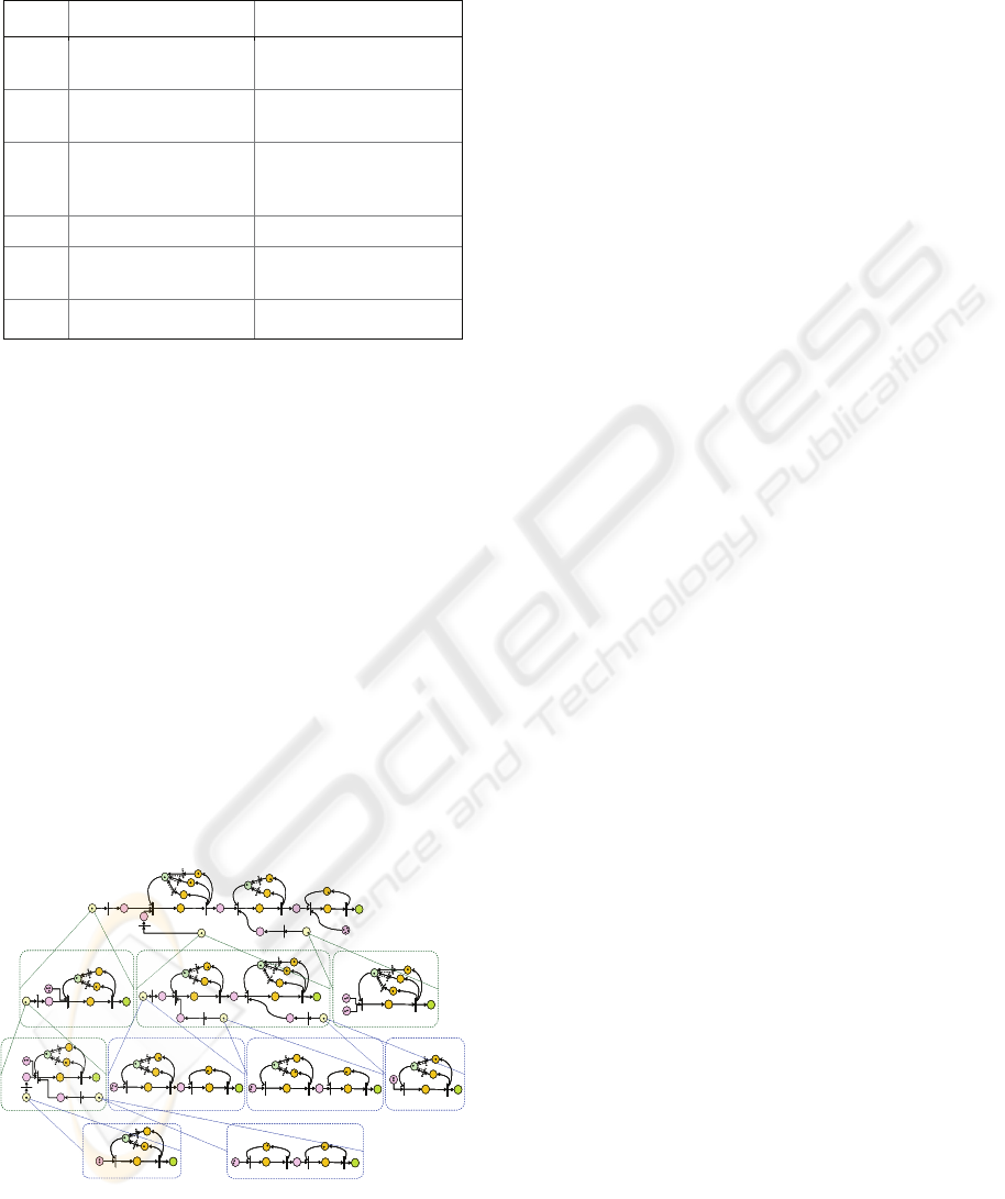
Table 3: The places, represented elements and colored
tokens/nets.
Places System Elements Colored Tokens
39
p
A raw material buffer
for Bas
(
)
{
}
1.Ba,1.Ba,1.Bap
32139
=
α
40
p
A conceptual machines
for manufacturing Bas
(){ }
131240
m,mp =
α
42/41
p
Alternative idle
machines for
manufacturing Bas
(
)
{
}
(
)
{
}
13421241
mp/mp ==
αα
… … …
46
p
The second machine
processing Ba WIPs
(){ }
32146
Ba,Ba,Bap =
α
47
p
A buffer for Bas
(){ }
32147
Ba,Ba,Bap =
α
PNet
is the process net describing the abstract
production processes of end-products;
{}
M
N
i
MNetM = is a finite set of MNets ; and
{}
A
N
i
ANetA =
is a finite set of ANets .
Performing as an abstraction mechanism,
MlNNS facilitates the configuration of processes
with right amount of details. Within
MlNNS , the
highest level is the
PNet
, while a number of MNets
and
ANets are located at the second level. Each of
these nets provides more details for processes of
input items involved in the
PNet
. At the lowest level
of each path, all nets are
MNets , whilst a mixture of
MNets and ANets can be found at any arbitrary
level.
For the motor family, based on the constructed
MNets , ANets and PNet , the multilevel system of
production configuration is obtained, as shown in
Figure 5.
22
p
29
p
15
t
20
t
31
p
23
p
25
p
24
p
16
t
17
t
23
t
34
p
36
p
25
t
33
p
22
t
37
p
26
t
38
p
30
p
21
t
32
p
18
t
27
p
28
p
19
t
26
p
24
t
35
p
1
p
9
p
1
t
7
t
10
p
2
p
4
p
3
p
2
t
3
t
4
t
6
p
8
p
6
t
5
p
9
t
16
p
13
t
17
p
11
p
8
t
12
p
10
t
14
p
15
p
11
t
13
p
18
p
5
t
7
p
19
p
20
p
21
p
14
t
PNet
60
p
62
p
41
t
57
p
56
p
58
p
37
t
38
t
63
p
39
t
61
p
40
t
59
p
familyAA
ofANet
familyBA
ofANet
48
p
49
p
33
t
51
p
53
p
35
t
50
p
32
t
54
p
36
t
55
p
34
t
52
p
familyFA
ofANet
54
t
87
p
57
t
79
p
82
p
83
p
53
t
56
t
88
p
85
p
55
t
84
p
81
p
80
p
86
p
52
t
family
CAof
ANet
27
t
43
p
30
t
44
p
39
p
28
t
41
p
42
p
29
t
40
p
45
p
46
p
47
p
32
t
31
t
familyBaofMNet
42
t
68
p
45
t
69
p
64
p
43
t
66
p
67
p
44
t
65
p
70
p
71
p
72
p
47
t
46
t
familyBbofMNet
75
p
48
t
77
p
51
t
78
p
73
p
49
t
76
p
50
t
74
p
family
TlofMNet
58
t
93
p
61
t
94
p
89
p
59
t
92
p
60
t
90
p
91
p
familyTp
ofMNet
62
t
97
p
63
t
98
p
95
p
96
p
99
p
100
p
101
p
65
t
64
t
familyClofMNet
22
p
29
p
15
t
20
t
31
p
23
p
25
p
24
p
16
t
17
t
23
t
34
p
36
p
25
t
33
p
22
t
37
p
26
t
38
p
30
p
21
t
32
p
18
t
27
p
28
p
19
t
26
p
24
t
35
p
22
p
29
p
15
t
20
t
31
p
23
p
25
p
24
p
16
t
17
t
23
t
34
p
36
p
25
t
33
p
22
t
37
p
26
t
38
p
30
p
21
t
32
p
18
t
27
p
28
p
19
t
26
p
24
t
35
p
1
p
9
p
1
t
7
t
10
p
2
p
4
p
3
p
2
t
3
t
4
t
6
p
8
p
6
t
5
p
9
t
16
p
13
t
17
p
11
p
8
t
12
p
10
t
14
p
15
p
11
t
13
p
18
p
5
t
7
p
19
p
20
p
21
p
14
t
PNet
1
p
9
p
1
t
7
t
10
p
2
p
4
p
3
p
2
t
3
t
4
t
6
p
8
p
6
t
5
p
9
t
16
p
13
t
17
p
11
p
8
t
12
p
10
t
14
p
15
p
11
t
13
p
18
p
5
t
7
p
19
p
20
p
21
p
14
t
PNet
60
p
62
p
41
t
57
p
56
p
58
p
37
t
38
t
63
p
39
t
61
p
40
t
59
p
familyAA
ofANet
60
p
62
p
41
t
57
p
56
p
58
p
37
t
38
t
63
p
39
t
61
p
40
t
59
p
60
p
62
p
41
t
57
p
56
p
58
p
37
t
38
t
63
p
39
t
61
p
40
t
59
p
familyAA
ofANet
familyBA
ofANet
48
p
49
p
33
t
51
p
53
p
35
t
50
p
32
t
54
p
36
t
55
p
34
t
52
p
familyFA
ofANet
48
p
49
p
33
t
51
p
53
p
35
t
50
p
32
t
54
p
36
t
55
p
34
t
52
p
48
p
49
p
33
t
51
p
53
p
35
t
50
p
32
t
54
p
36
t
55
p
34
t
52
p
familyFA
ofANet
54
t
87
p
57
t
79
p
82
p
83
p
53
t
56
t
88
p
85
p
55
t
84
p
81
p
80
p
86
p
52
t
family
CAof
ANet
27
t
43
p
30
t
44
p
39
p
28
t
41
p
42
p
29
t
40
p
45
p
46
p
47
p
32
t
31
t
familyBaofMNet
27
t
43
p
30
t
44
p
39
p
28
t
41
p
42
p
29
t
40
p
45
p
46
p
47
p
32
t
31
t
27
t
43
p
30
t
44
p
39
p
28
t
41
p
42
p
29
t
40
p
45
p
46
p
47
p
32
t
31
t
familyBaofMNet
42
t
68
p
45
t
69
p
64
p
43
t
66
p
67
p
44
t
65
p
70
p
71
p
72
p
47
t
46
t
familyBbofMNet
42
t
68
p
45
t
69
p
64
p
43
t
66
p
67
p
44
t
65
p
70
p
71
p
72
p
47
t
46
t
42
t
68
p
45
t
69
p
64
p
43
t
66
p
67
p
44
t
65
p
70
p
71
p
72
p
47
t
46
t
familyBbofMNet
75
p
48
t
77
p
51
t
78
p
73
p
49
t
76
p
50
t
74
p
family
TlofMNet
75
p
48
t
77
p
51
t
78
p
73
p
49
t
76
p
50
t
74
p
75
p
48
t
77
p
51
t
78
p
73
p
49
t
76
p
50
t
74
p
family
TlofMNet
58
t
93
p
61
t
94
p
89
p
59
t
92
p
60
t
90
p
91
p
familyTp
ofMNet
58
t
93
p
61
t
94
p
89
p
59
t
92
p
60
t
90
p
91
p
58
t
93
p
61
t
94
p
89
p
59
t
92
p
60
t
90
p
91
p
familyTp
ofMNet
62
t
97
p
63
t
98
p
95
p
96
p
99
p
100
p
101
p
65
t
64
t
familyClofMNet
62
t
97
p
63
t
98
p
95
p
96
p
99
p
100
p
101
p
65
t
64
t
62
t
97
p
63
t
98
p
95
p
96
p
99
p
100
p
101
p
65
t
64
t
familyClofMNet
Figure 5: The multilevel nested net system of production
configuration.
As shown in the figure, the PNet is at the
highest level; 3
ANets for producing assembly
families AA, BA and FA are located at the second
level; 1
ANet for producing CA family and 3 MNets
for manufacturing part families Ba, Bb and Tl are at
the third level; and 2
MNets for fabricating part
families Tp and Cl are located at the lowest level.
Each lower level nested net is linked with the
corresponding tokens residing in the places of the
higher level nets.
4.2 System Evolution
Complying with production practice, in the
MlNNS ,
MNets nest in places of ANets and/or
PNet
; and
ANets nest in places of higher level ANets and/or
PNet
. Consequently, configuration of a complete
production process for an end-product necessitates
interaction of the nested nets and the host nets. In
this study, transition synchronization is introduced to
enable interaction of nets at different levels.
Transition synchronization is declared by the color
pairs/triples of net transitions. More specifically, two
or more transitions with same color pairs and/or
triples must be synchronized, i.e., fire
simultaneously. To enable transition
synchronization, several rules for enabling and firing
transitions are defined in the net system.
Rule 1: A transition,
t
, of an MNet is enabled
with respect to a color pair,
cp , and fires
autonomously without additional conditions if
(
)
(
)
(
)
pcp,t,p,p
μΕ
⊆∀
and
(
)
εΣ
,cp
M
= .
Rule 2: A transition,
t
, of an MNet is enabled
and fires simultaneously with an output transition of
the place, where the
MNet is nested, of the higher
level
ANet or PNet if
()()()
pcp,t,p,p
μ
Ε
⊆
∀
and
(
)
MM
,cp
ΣΣ
= .
Rule 3: A transition,
t , of an ANet is enabled
with respect to a color triple,
ct , and fires
autonomously without additional conditions if
(
)
(
)
(
)
pct,t,p,p
μΕ
⊆∀
and
(
)
εΣε
,,ct
A
= .
Rule 4: A transition,
t
, of an ANet is enabled
and fires simultaneously with a transition bearing a
(
)
AA
,cp
ΣΣ
= or
(
)
AA
,,ct
ΣΣε
= of the lower level
MNet or ANet that nests in an input place of t , if
(
)
(
)
(
)
pct,t,p,p
μ
Ε
⊆
∀
and
(
)
εΣΣ
,,ct
AA
= .
Rule 5: A transition,
t , of an ANet is enabled
and fires simultaneously with an output transition of
a place, where the
ANet is nested, of the higher
level
ANet or PNet , if
()()()
pct,t,p,p
μ
Ε
⊆
∀
and
(
)
AA
,,ct
ΣΣε
=
.
Rule 6: A transition,
t , of a PNet is enabled
with respect to a color pair,
cp , and fires
ICEIS 2008 - International Conference on Enterprise Information Systems
10

autonomously without additional conditions if
()()()
pcp,t,p,p
μΕ
⊆∀ and
(
)
P
,cp
Σε
= .
Rule 7: A transition,
t
, of a PNet is enabled and
fires simultaneously with a transition bearing a
(
)
MM
,cp
ΣΣ
= or
(
)
AA
,,ct
ΣΣε
= of the lower level
MNet or ANet that nests in an input place of t , if
()()()
pcp,t,p,p
μ
Ε
⊆∀ and
(
)
PP
,cp
ΣΣ
= .
While the firing of transitions of any net does not
provoke the transfer of nested nets, that is, the nested
nets remain in the same places before and after
simultaneous transition firing, the tokens, other than
the nested nets, are created and removed as follows:
Rule 8: The firing of an enabled transition,
t
, in
nets at all levels modifying the marking through 1)
generating tokens in the output places by following
()()
cp,p,t
Ε
or
()()
ct,p,t
Ε
; and 2) removing tokens
in the input places by following
()()
cp,t,p
Ε
or
()()
ct,t,p
Ε
.
5 APPLICATION RESULTS
For the 3 motor variants:
21
VM,VM and
3
VM in
Figure 3 and Table 1, more than one production
process consisting of different combination of
machines is feasible to fulfil each motor variant. In
this regard, minimizing the completion time of the
last operation of producing three motor variants is
chosen as the production objective and, the selection
of appropriate ones is made based on this objective.
In the application, we adopt the shortest delay times
to fire transitions, which are enabled by alternative
colored tokens. Table 5 list the corresponding
processes with respect to the selected machines. Due
to the space constraints, this table is truncated.
6 CONCLUSIONS
This study addresses the logic for configuring
production processes of product families with an
attempt to assist practitioners to better understand
and implement production configuration. In view of
the significance of PN techniques in modelling
complex systems/processes, we propose a formalism
of NCTPNs to model production configuration. By
integrating the basic principles of several well-
defined PN extensions, the NCTPNs are able to
capture and reflect the complex process of
configuring complete production processes for end
products. The industrial example has shown
Table 5: The configured production processes for the 3
motor variants.
Machine(Operation; Output item)
1
VM
2
VM
3
VM
13
m (Manufacturing
operation;
1
Ba )
13
m (Manufacturing
operation;
2
Ba )
12
m (Manufacturing
operation;
3
Ba )
14
m (Manufacturing
operation;
1
Ba )
14
m (Manufacturing
operation;
2
Ba )
14
m (Manufacturing
operation;
2
Ba )
… … …
5
m
(Assembly
operation;
1
MB )
5
m
(Assembly
operation;
2
MB )
4
m (Assembly
operation;
3
MB )
6
m (Assembly
operation;
1
VM )
6
m (Assembly
operation;
2
VM )
6
m (Assembly
operation;
3
VM )
the potential of the NCTPNs formalism to reveal the
logic of production configuration.
REFERENCES
Dash, S., Kalagnanam, J., Reddy, C., Song, S.H., 2007.
Production design for plate products in the steel
industry, IBM Journal of Research & Development,
51, 354-362.
Jensen, K., 1995. Colored Petri nets: Basic concepts,
analysis methods and practical Use
. Vol. 2, New
York, Springer.
Lomazova, I.A., 2000. Nested Petri nets: A formalism for
specification and verification of multi-agent
distributed systems, Fundamenta Informaticae, 43,
195-214.
Martinez, M.T., Favrel, J., Ghodous, P., 2000. Product
family manufacturing plan generation and
classification, Concurrent Engineering: Research and
Applications
, 8, 12-22.
Peterson, J.L., 1981.
Petri net theory and the modelling of
Systems, Prentice-Hall, Englewood Cliffs, N.J.
Ramachandani, C., 1974. Analysis of asynchronous
concurrent systems by timed Petri nets, Technical
Report MAC TR 120, MIT, Cambridge.
Schierholt, K., 2001. Process configuration: Combining
the principles of product configuration and process
planning, Artificial Intelligence for Engineering
Design, Analysis and Manufacturing
, 15, 411-424.
Zhang, L., 2007. Process Platform-based Production
Configuration for Mass Customization, PhD
Dissertation, Division of Systems and Engineering
Management, Nanyang Technological University,
Singapore.
Zhang, L., Jiao, J., Helo, P., 2007. Process platform
representation based on unified modelling language,
International Journal of Production Research, 45,
323-350.
PRODUCTION CONFIGURATION OF PRODUCT FAMILIES - An Approach based on Petri Nets
11
