
Discr
ete-Time Drift Counteracting Stochastic Optimal
Control and Intelligent Vehicle Applications
Ilya Kolmanovsky and John Michelini
Ford Research and Advanced Engineering, Ford Motor Company
2101 Village Road, Dearborn, Michigan, U.S.A.
Abstract. In this paper we present a characterization of a stochastic optimal
control in the problem of maximizing expected time to violate constraints for
a nonlinear discrete-time system with a measured (but unknown in advance) dis-
turbance modeled by a Markov chain. Such an optimal control may be viewed as
providing drift counteraction and is, therefore, referred as the drift counteracting
stochastic optimal control. The developments are motivated by an application to
an intelligent vehicle which uses an adaptive cruise control to follow a randomly
accelerating and decelerating vehicle. In this application, the control objective is
to maintain the distance to the lead vehicle within specified limits for as long
as possible with only gradual (small) accelerations and decelerations of the fol-
lower vehicle so that driver comfort can be increased and fuel economy can be
improved.
1 Introduction
In the paper we examine a stochastic optimal control problem motivated by an appli-
cation of adaptive cruise control to follow a randomly accelerating and decelerating
vehicle. For this application, we consider the control objective to maintain the distance
to the lead vehicle within specified limits for as long as possible with only very gradual
(small) accelerations and decelerations so that to improve fuel economy and increase
driver comfort. This and similar application problems can be treated using methods of
stochastic drift counteracting optimal control developed in [6].
The paper is organized as follows. In Section 2 we discuss a formulation of the
stochastic drift counteracting optimal control problem for a nonlinear discrete-time sys-
tem with measured (but unknown in advance) disturbance input modeled by a Markov
chain. In Section 3 we review the theoretical results [6] pertinent to the characterization
and computations of the stochastic optimal control law in this problem. We also present
a result to compute expected time to violate the constraints for a fixed control policy,
which may be useful in evaluating legacy control solutions. In Section 4 we discuss a
simulation example illustrating the application of these methods to a vehicle follow-
ing, where the lead vehicle speed trajectory is modeled by a Markov chain with known
transition probabilities. Concluding remarks are made in Section 5.
Kolmanovsky I. and Michelini J. (2008).
Discrete-Time Drift Counteracting Stochastic Optimal Control and Intelligent Vehicle Applications.
In Proceedings of the 2nd International Workshop on Intelligent Vehicle Control Systems, pages 7-16
Copyright
c
SciTePress
2 Problem Formulation
Consider a system which can be modeled by nonlinear discrete-time equations,
x(t + 1) = f (x(t), v(t), w(t)), (1)
where x(t) is the state vector, v(t) is the control vector, w(t) is the vector of measured
disturbances, and t is an integer, t ∈ Z
+
. The system has control constraints which are
expressed in the form v(t) ∈ U, where U is a given set.
The behavior of w(t) is modeled by a Markov chain [3] with a finite number of
states w(t) ∈ W = {w
j
, j ∈ J}. The transition probability from w(t) = w
i
∈ W to
w(t + 1) = w
j
∈ W is denoted by P (w
j
|w
i
, ¯x). In our treatment of the problem, we
permit this transition probability to depend on the state x(t) = ¯x. For automotive appli-
cations, modeling driving conditions using Markov chains for the purpose of applying
Stochastic Dynamic Programming to determine fuel and emissions optimal powertrain
operating policies has been first proposed in [4].
Our objective is to determine a control function u(x, w), such that with v(t) =
u(x(t), w(t)), a cost functional of the form,
J
x
0
,w
0
,u
= E
x
0
,w
0
τ
x
0
,w
0
,u
(G),
(2)
is maximized. Here τ
x
0
,w
0
,u
(G) ∈ Z
+
denotes the first-time instant the trajectory of
x(t) and w(t), denoted by {x
u
, w
u
}, resulting from the application of the control v(t) =
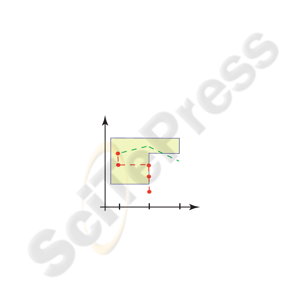
u(x(t), w(t)), exits a prescribed compact set G. See Figure 1.
w
1
w
2
w
3
w
x
*
*
*
t=0
t=1
t=2
t=3
t=4
t=1
t=2
|
G
|
|
Fig.1. The set G and two trajectories, {x
u
, w
u
}, exiting G at random time instants due to a
random realization of w(t). Here W = {w
1
, w
2
, w
3
}. Note that one of the trajectories exits G
at t = 4 due to the evolution of x(t) alone, the other trajectory exits G at t = 2 due to evolution
of both x(t) and w(t).
The specification of the set G reflects constraints existing in the system. Note that
{x
u
, w
u
} is a random process, τ
x
0
,w
0
,u
(G) is a random variable and E
x
0
,w
0
[·] denotes
8

the expectation conditional to initial values of x and w, i.e., x(0) = x
0
, w(0) = w
0
.
When clear from the context, we will omit the subscript and square brackets around E.
For continuous-time systems, under an assumption that w(t) is a Wiener or a Pois-
son process, it can be shown [1] that determining an optimal control in this kind of a
problem reduces to solving a non-smooth Partial-Differential Equation (PDE). For in-
stance, for a first order stochastic system, dx = (v − w
0
)dt + σ · dw, where w
0
is a
constant, w is a standard Wiener process, the control v satisfies |v| ≤ ¯v, this PDE has
the form,
1
2
σ
2
∂
2
V
∂x
2
+
∂V
∂x
(−w
0
) + |
∂V
∂x
|¯v + 1 = 0.
The boundary conditions for this PDE are V (x) = 0 for x ∈ ∂G, where ∂G denotes
the boundary of G. The optimal control has the form
v = ¯v · sign(
∂V
∂x
).
Note that this optimal control is of bang-bang type.
As compared to solving the above PDE numerically, the discrete-time treatment
of the problem, which is the focus of the present paper, appears to provide a more
computationally tractable approach to determining the optimal control. In what follows,
we will treat this discrete-time optimal control problem within the framework of optimal
stopping [3] and drift counteraction [5], [6] stochastic optimal control.
3 Theoretical Results and Computations
Given a state vector, x
−
, and disturbance vectors, w
−
, w
+
∈ W , we define,
L
u
V (x
−
, w
−
)
∆
= E
x
−
,w
−
·
V (f(x
−
, u(x
−
, w
−
), w
−
), w
+
)
¸
− V (x
−
, w
−
)
=
X
j∈J
V (f(x
−
, u(x
−
, w
−
), w
−
), w
j
) · P (w
j
¯
¯
w
−
, x
−
) (3)
− V (x
−
, w
−
).
The following theorem provides sufficient conditions for the optimal control law, u
∗
(x, w):
Theorem 1: Suppose there exists a control function u
∗
(x, w) and a continuous, non-
negative function V (x, w) such that
L
u
∗
V (x, w) + 1 = 0, if (x, w) ∈ G,
L
u
V (x, w) + 1 ≤ 0, if (x, w) ∈ G, u 6= u
∗
,
V (x, w) = 0, if (x, w) 6∈ G.
(4)
Then, u
∗
maximizes (2), and for all (x
0
, w
0
) ∈ G, V (x
0
, w
0
) = J
x
0
,w
0
,u
∗
, J
x
0
,w
0
,u
and E[τ
x
0
,w
0
,u
(G)] are finite for any policy u, and the function V , satisfying (4), if
exists, is unique.
9

Proof: The theorem follows as an immediate application of a more general result
developed in [6]. More specifically, in [6], a similar result is shown for cost functionals
of the form
J
x
0
,w
0
,u
= E
x
0
,w
0
τ
x
0
,w
0
,u
(G)−1
X
t=0
g(x(t), v(t), w(t)),
with g ≥ ε > 0, of which (2) is a special case with g = 1. ¥
The following procedure for estimating the expected time to violate constraints for
a fixed control law is obtained as an immediate consequence of Theorem 1:
Corollary 1: Given a fixed control law ¯u(x, w), suppose there exists a continuous,
non-negative function
¯
V (x, w) such that
L
¯u
¯
V (x, w) + 1 = 0, if (x, w) ∈ G,
¯
V (x, w) = 0, if (x, w) 6∈ G.
(5)
Then, E[τ
x
0
,w
0
,¯u
(G)] =
¯
V (x
0
, w
0
).
We next consider the application of the value iteration approach to (4), assuming,
for simplicity of exposition, that f is continuous in x, and that U is compact. The
proofs of subsequent results are similar to [6,5] and are not reproduced here. We define
a sequence of value functions using the following iterative process:
V
0
≡ 0
V
n
(x, w
i
) = max
v∈U
½
X
j∈J
V
n−1
(f(x, v, w
i
), w
j
)P (w
j
|w
i
, x) + 1
¾
, if (x, w
i
) ∈ G.
n > 0.
(6)
This sequence of functions {V
n
} yields the following properties:
Theorem 2: Suppose the assumptions of Theorem 1 hold. Then the sequence of
functions {V
n
}, defined in (6), is monotonically non-decreasing and V
n
(x, w
i
) ≤ J
x,w
i
,u
∗
for all n, x and w
i
. Furthermore, {V
n
} converges pointwise to V
∗
(x, w
i
) = J
x,w
i
,u
∗
and this convergence is uniform if J
x,w
i
,u
∗
is continuous.
On the computational side, either value iterations or Linear Programming may be
used to numerically approximate the solution to (4).
The value iterations (6) produce a sequence of value function approximations, V
n
,
at specified grid-points x ∈ {x
k
, k ∈ K}, and a stopping criterion is |V
n
(x, w
i
) −
V
n−1
(x, w
i
)| ≤ ² for all x ∈ {x
k
, k ∈ K} and i ∈ J, where ² > 0 is sufficiently small.
In each iteration, once the values of V
n−1
at the grid-points have been determined, linear
or cubic interpolation may be employed to approximate V
n−1
(f(x
k
, v
m
, w
i
), w
j
), on
the right-hand side of (6), where v ∈ {v
m
, m ∈ M} is a specified grid for v. Formally,
the approximate value iterations can be represented as follows,
V
0
(x
k
, w
i
) ≡ 0,
V
n
(x
k
, w
i
) = max
v
m
,m∈M
½
X
j∈J
F
n−1
(f(x
k
, v
m
, w
i
), w
j
) · P (w
j
|w
i
, x
k
) + 1
¾
,
where
F
n−1
(x, w
i
) = Interpolant[V
n−1
](x, w
i
) if (x, w
i
) ∈ G,
and F
n−1
(x, w
i
) = 0 if (x, w
i
) 6∈ G.
(7)
10

An alternative approach is to seek V in the form,
V (x, w
i
) =
X
l∈L
θ
l
φ
l
(x, w
i
),
where φ
l
are specified basis functions satisfying the property that φ
l
(x, w
i
) = 0 if
(x, w
i
) 6∈ G. Then relations (4) evaluated over specified grid points x ∈ {x
k
, k ∈ K},
v ∈ {v
m
, m ∈ M }, and i ∈ J, lead to a Linear Programming problem with respect to
θ
l
, l ∈ L:
X
l∈L
θ
l
X
k∈K,i∈J
φ
l
(x
k
, w
i
) → min,
subject to
X
l∈L
θ
l
φ
l
(x
k
, w
i
) ≥ 1 +
X
l∈L
θ
l
X
j∈J
φ
l
(f(x
k
, v
m
, w
i
), w
j
) · P (w
j
|w
i
, x
k
),
k ∈ K, i ∈ J, m ∈ M.
(8)
There are many aspects, such as selection of the grids and basis functions, which can
be exploited to optimize the computations for specific problems. The dependence of the
approximation error on the properties of the grid can be established using, for instance,
techniques in Chapter 16 of [2].
Once an approximation of the value function, V
∗
, is available, an optimal control
may be determined from the following relation:
u
∗
(x, w
i
) ∈ argmax
v∈ U
½
1 +
X
j∈J
V
∗
(f(x, v, w
i
), w
j
)P (w
j
|w
i
, x)
¾
,
or
u
∗
(x, w
i
) ∈ argmax
v∈ U
½
X
j∈J
V
∗
(f(x, v, w
i
), w
j
)P (w
j
|w
i
, x)
¾
. (9)
4 Vehicle Following Example
In this section we illustrate the above developments with an example of an intelligent
vehicle which uses an adaptive cruise control to follow another, randomly accelerating
and decelerating vehicle. In this application, the control objective is to maintain the
distance to the lead vehicle within specified limits for as long as possible with only very
gradual (small) accelerations and decelerations of the follower vehicle to improve fuel
economy and increase driver comfort.
The relative distance between two vehicles minus minimum acceptable distance is
denoted by s [m], the velocity of the lead vehicle is denoted by v
l
[mph], the velocity
of the follower vehicle is denoted by v
f
[mph] and ∆T is the sampling time period.
Assuming that the acceleration a [mph/sec] of the follower vehicle is a control variable,
the discrete-time update equations have the following form,
s(t + 1) = s(t) + 0.1736 · ∆T · (v
l
(t) − v
f
(t)),
v
f
(t + 1) = v
f
(t) + ∆T · a(t). (10)
11
The factor 0.1736 is introduced because the velocity units are in miles-per-hour (mph)
while the distance is in meters (m). With x = [s, v
f
]
T
, w = v
l
, and v = a as the control,
(10) has the form of (1).
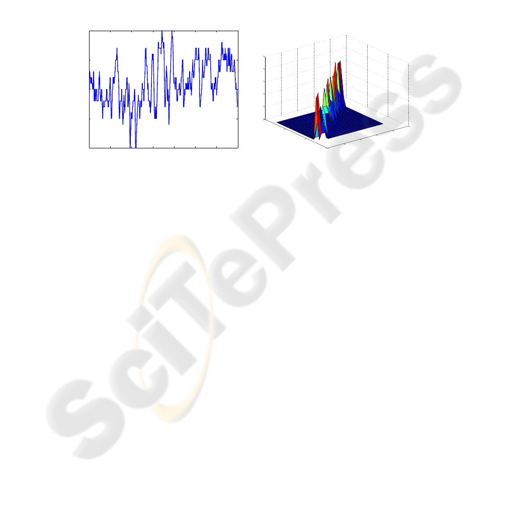
We consider a scenario when the vehicles are driven on a road with average speed of
55 mph, minimum speed of 46 mph and maximum speed of about 66 mph. The update
period is fixed to ∆T = 1 sec. The lead vehicle velocity, w = v
l
, is modeled by a
Markov chain with 20 discrete levels uniformly distributed between 46 and 66.0013
mph. The transition probabilities (see Figure 2-right) have been constructed from an
experimental vehicle velocity trajectory shown in Figure 2-left.
0 200 400 600 800 1000 1200 1400
45
50
55
60
65
t
v
l
[mph]
45
50
55
60
65
70
40
50
60
70
0
0.2
0.4
0.6
0.8
1
future v
l
[mph]
current v
l
[mph]
p
i,j
Fig.2. Left: Experimental vehicle velocity trajectory. Right: Transition probabilities of the
Markov chain model of the lead vehicle velocity.
It is desired to maintain the relative distance between two vehicles minus minimum
acceptable distance in the range s ∈ [0, 20] meters. The accelerations of the follower
vehicle must be in the range a ∈ [−0.5, 0.5] mph/sec.
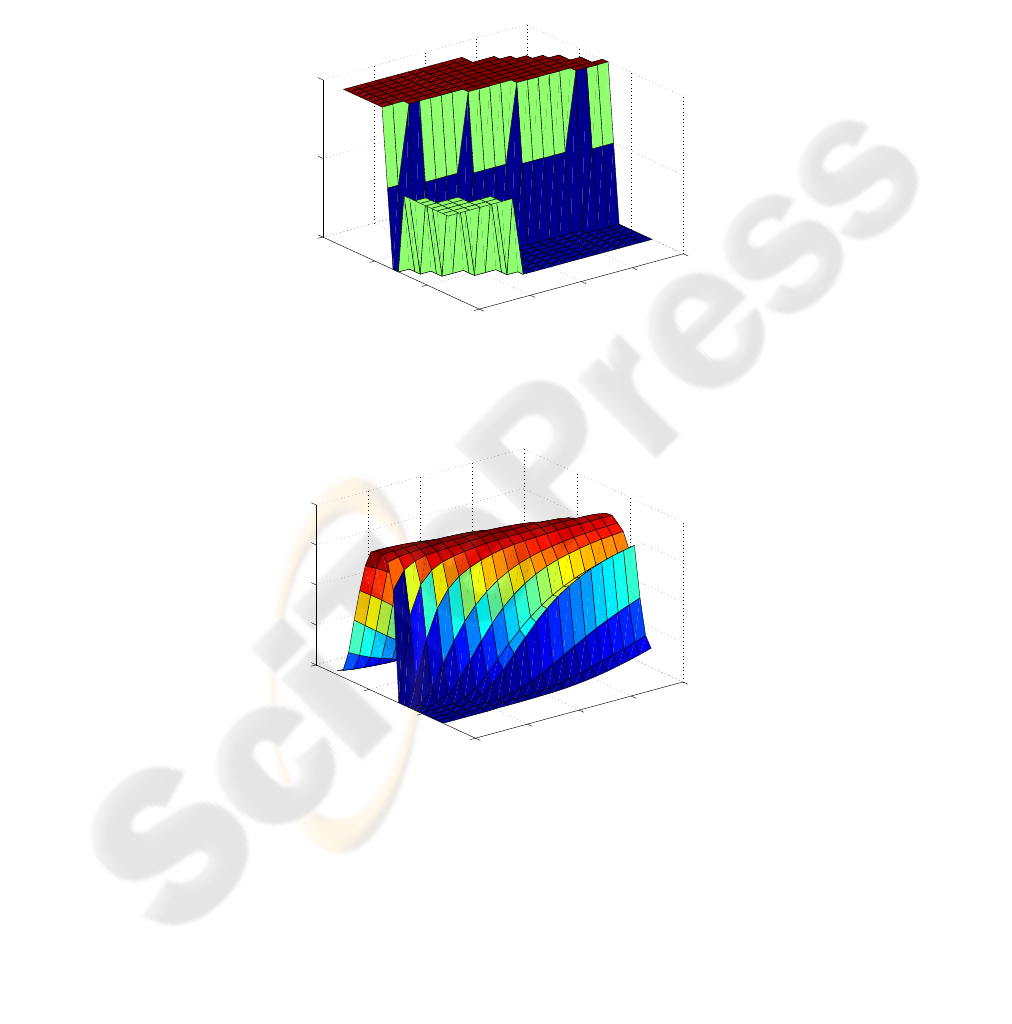
An approximation of the optimal control, u
∗
, determined using the value itera-
tion approach, is illustrated in Figure 3 while the value function, V
∗
is illustrated in
Figure 4. Note that the u
∗
and V
∗
depend on three variables: s, v
f
, and v
l
. Hence,
only the cross-sections of u
∗
and V
∗
are shown for a fixed value of v
f
. Figure 5
demonstrates numerically the convergence of the value iterations. The grids used were
{−0.5, −0.25, 0, 0.25, 0.5} for a, {46, 47.0527, 48.1054, ··· , 66.0013} for v
f
and v
l
,
and {0, 1.0526, 2.1053, ··· , 20} for s.
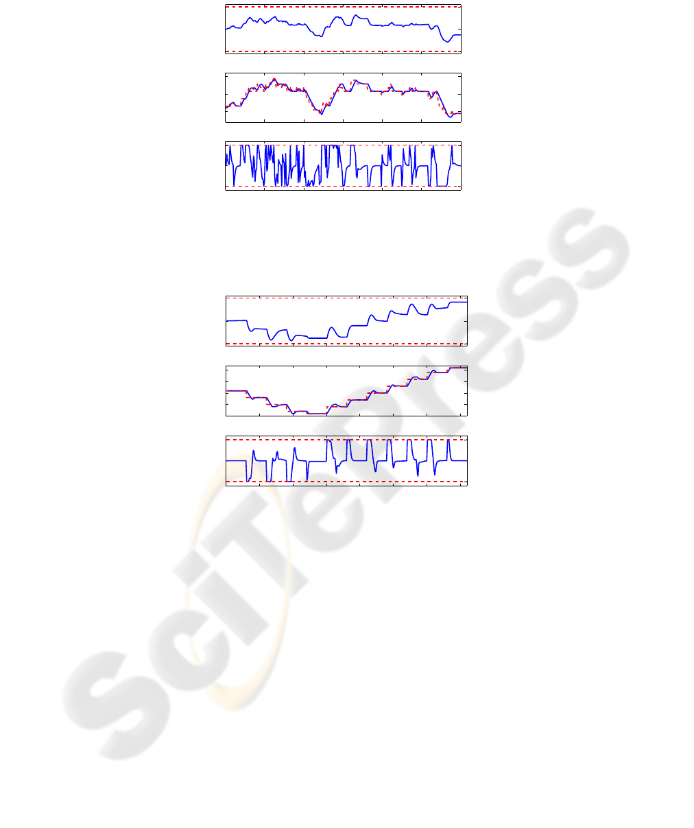
Figures 6 illustrates the time responses when the follower vehicle is controlled with
the above approximate stochastic optimal control and when the lead vehicle velocity
is a typical realization of the Markov chain trajectory. Note that the accelerations and
decelerations of the lead vehicle are up to 2.1 mph/sec, well in excess of 0.5 mph/sec
limit imposed on the accelerations and decelerations of the follower vehicle. Figure 7 il-
lustrates the time responses when the lead vehicle velocity is a sequence of non-random
accelerations and decelerations.
As can be observed from the plots, the velocity of the follower vehicle, controlled
by stochastic drift counteracting optimal control, tracks the velocity of the lead vehicle
but with smaller accelerations and decelerations, which satisfy the required limits of 0.5
12
mph/sec. The controller also enforces the constraints on the relative distance between
the vehicles. When the lead vehicle moves at high speed, the follower vehicle increases
the relative distance knowing that deceleration of the lead vehicle is more likely and
acceleration is less likely. When the lead vehicle moves at low speed, the follower vehi-
cle decreases the relative distance knowing that acceleration of the lead vehicle is more
likely and deceleration is less likely. This behavior of the follower vehicle is direction-
ally consistent with the constant headway time policy.
0
5
10
15
20
40
50
60
70
−0.5
0
0.5
Relative distance [m]
Follower Vehicle Vel=55.4743
Lead vehicle [mph]
u
*
Fig.3. A cross-section of approximate optimal control.
0
5
10
15
20
40
50
60
70
0
100
200
300
400
Relative distance [m]
Follower Vehicle Vel=55.4743
Lead vehicle [mph]
Optimal E[τ]
Fig.4. A cross-section of approximate optimal value function.
Remark 1: The stochastic optimal control maximizes the expected time to violate
the constraints, but it cannot entirely eliminate the possibility that the constraints are
violated. If the relative distance constraints become violated, a decision needs to be
13
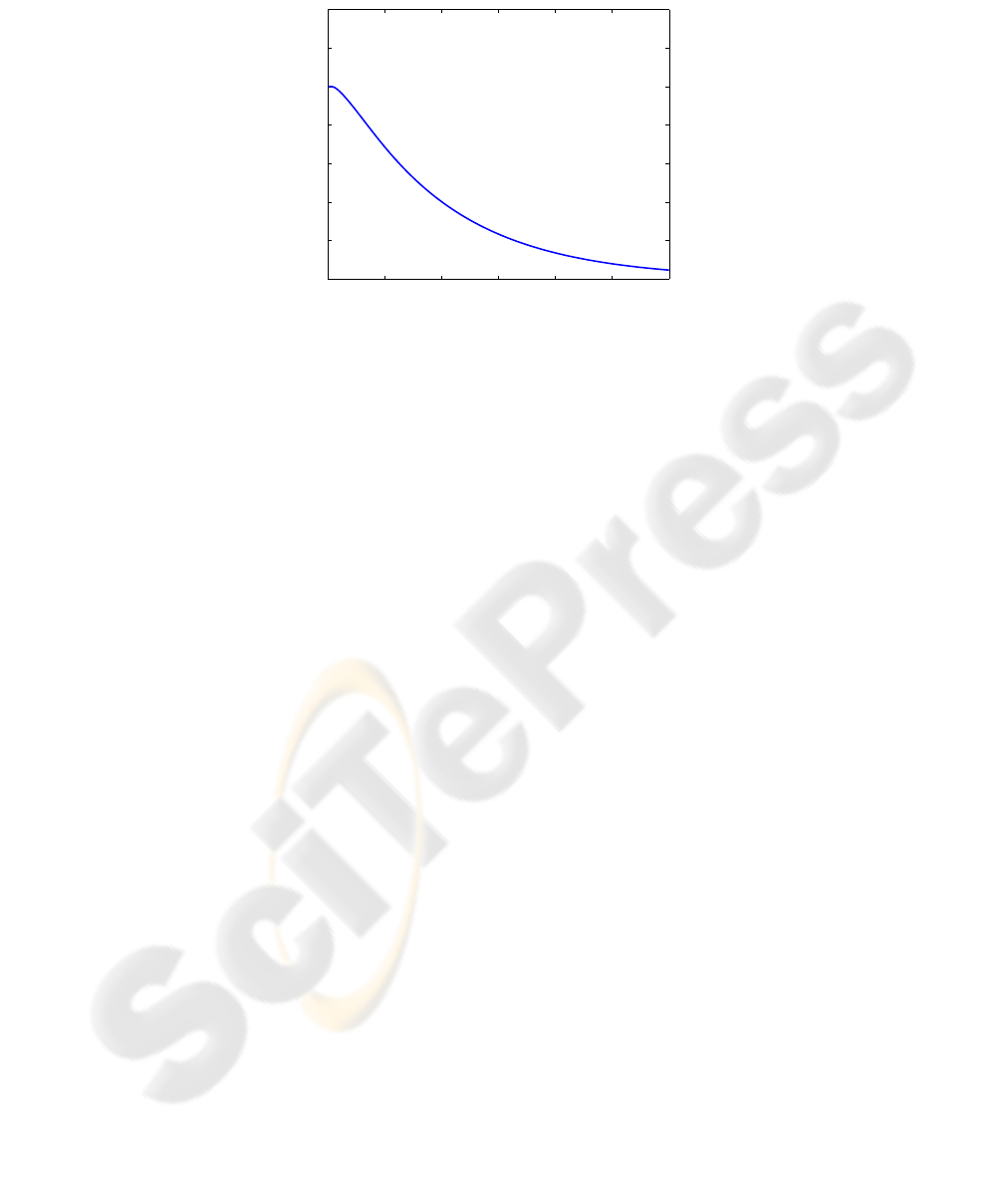
0 200 400 600 800 1000 1200
0
0.2
0.4
0.6
0.8
1
1.2
1.4
Iteration
max |V
n
−V
n−1
|
Fig.5. Maximum of |V
n
(x, w
i
) − V
n−1
(x, w
i
)| over x ∈ {x
k
, k ∈ K} and i ∈ J as the value
iterations progress (i.e., n increases).
made if to discontinue following the lead vehicle since it is too difficult to follow, or
to switch to a different controller which may use larger accelerations and decelerations
to bring the relative distance and the follower vehicle velocity to values appropriate to
re-engage the stochastic optimal controller.
Remark 2: The transition probabilities for the lead vehicle velocity may be estimated
on-line by measuring the lead vehicle velocity. Considering that on-board computing
power may be limited, fast procedures to approximate u
∗
, once transition probabilities
have been estimated, are desirable. The development of such procedures is a subject of
future research.
5 Concluding Remarks
In this paper we presented a method for constructing a stochastic optimal control law in
the problem of maximizing expected time to violate constraints for a nonlinear discrete-
time system with a measured (but unknown in advance) disturbance modeled by a
Markov chain. The resulting control law is referred to as the stochastic drift counter-
acting optimal control law.
A simulation example was considered where an intelligent vehicle follows another,
randomly accelerating and decelerating lead vehicle. The control objective in this ex-
ample was to control the follower vehicle acceleration to maintain the distance to the
lead vehicle within specified limits and avoid high accelerations and decelerations so
as to improve fuel economy and increase driver comfort. It has been shown that the
behavior of the vehicle with the stochastic drift counteracting optimal control law is
intuitively reasonable, e.g., the relative distance between the vehicles increases (respec-
tively, decreased) when the lead vehicle is near its maximum (respectively, minimum)
speed, as the follower vehicle expects a deceleration (respectively, acceleration) of the
lead vehicle.
14
0 50 100 150 200 250 300
0
10
20
s
0 50 100 150 200 250 300
55
60
65
v
f
, v
l
[r−−]
0 50 100 150 200 250 300
−0.5
0
0.5
a
t
Fig.6. Relative distance (top), follower and lead vehicle velocities (middle) and follower vehicle
acceleration (bottom) in response to random lead vehicle velocity profile. Relative distance con-
straints and acceleration constraints are indicated on the top plot and bottom plot, respectively,
by dashed lines. Dashed lines in the middle plot indicate the lead vehicle velocity.
0 50 100 150 200 250 300 350
0
10
20
s
0 50 100 150 200 250 300 350
45
50
55
60
65
v
f
, v
l
[r−−]
0 50 100 150 200 250 300 350
−0.5
0
0.5
a
t
Fig.7. Relative distance (top), follower and lead vehicle velocities (middle), and follower vehicle
acceleration (bottom) in response to non-random lead vehicle velocity profile. Relative distance
constraints and acceleration constraints are indicated on the top plot and bottom plot, respectively,
by dashed lines. Dashed lines in the middle plot indicate the lead vehicle velocity.
More elaborate vehicle models and lead vehicle speed models can be treated simi-
larly even though, as with any dynamic programming approach, high state dimensions
present an obstruction due to “curse of dimensionality.” Fast procedures for comput-
ing or approximating the stochastic optimal control law, so that it can be reconfigured
on-line if the problem parameters or statistical properties of the lead vehicle veloc-
ity change, is a subject of future research. While this paper only discussed procedures
suitable for off-line computations, these results are already valuable as the resulting
stochastic optimal control law can be used as a benchmark for control algorithms de-
veloped other approaches, and it can yield valuable insights into the optimal behavior
15

desirable of the follower vehicle. Also, from Figure 3, it appears that u
∗
does not have
a very elaborate form and so it may inspire a simpler rule-based control law which
achieves a near optimal performance.
The theoretical results and computational approaches discussed in this paper can
have other applications in intelligent vehicle control and manufacturing. Specifically,
they may be applicable in other situations where there is a disturbance with statistical
properties that can be modeled in advance (e.g., demands of the driver, changes in the
environmental conditions, production orders being scheduled, etc.) while pointwise-in-
time constraints on certain critical state and control variables need to be enforced. Along
these lines, another example application to Hybrid Electric Vehicle (HEV) control has
been discussed in [6].
References
1. Afanas’ev, V.N., Kolmanovskii, V.B., and Nosov, V.R. (1996). Mathematical Theory of Con-
trol Systems Design. Kluwer Academic Publishers.
2. Altman, E. (1999). Constrained Markov Decision Processes. Chapman and Hall/CRC.
3. Dynkin, E.B., and Yushkevich, A.A. (1967). Markov Processes: Theorems and Problems.
Nauka, Moscow, in Russian. English translation published by Plenum, New York, 1969.
4. Kolmanovsky, I., Sivergina, I., and Lygoe, B. (2002). Optimization of powertrain operat-
ing policies for feasibility assessment and calibration: Stochastic dynamic programming ap-
proach. Proceedings of 2002 American Control Conference. Anchorage, AK, pp. pp. 1425–
1430.
5. Kolmanovsky, I., and Maizenberg, T.L. (2002). Optimal containment control for a class of
stochastic systems perturbed by Poisson and Wiener processes. IEEE Transactions on Auto-
matic Control. Vol. 47, No. 12, pp. 2041–2046.
6. Kolmanovsky, I., Lezhnev, L., and Maizenberg, T.L. (2008). Discrete-time drift counterac-
tion stochastic optimal control: Theory and application-motivated examples. Automatica,
Vol. 44 , No. 1, pp. 177–184.
16
