Intelligent

Refueling Advisory System

Erica Klampﬂ

, Oleg Gusikhin

, Kacie Theisen

, Yimin Liu

and T. J. Giuli

Ford Research & Advanced Engineering, Systems Analytics & Environmental Sciences

Department, RIC Bldg, MD #2122, 2101 Village Rd., Dearborn, MI 48124, U.S.A.

Ford Research & Advanced Engineering, Vehicle Design & Infotronics Department

RIC Bldg, MD #3137, 2101 Village Rd., Dearborn, MI 48124, U.S.A.

Abstract. Recent advances in wireless communication technologies have led to

numerous new developments that take advantage of network access, ranging from

real-time information delivery essential for many driving decisions to harvesting

off-board computing power for remote vehicle diagnostics. Speciﬁcally, with the

ever increasing fuel cost, there is growing popularity of services that provide

information to drivers on current gas prices and alerts on upcoming changes to

gas prices. This paper demonstrates how to take currently available technology

one step further by providing a proactive refueling advisory system based on

minimizing fuel costs over routes and time. The system integrates vehicle data, a

navigation system, and internet connectivity to supplant the existing vehicle low

fuel warning with a comprehensive decision support system on refueling choices.

1 Introduction

Recent advances in wireless communication technologies have led to numerous devel-

opments that take advantage of internet connectivity. These developments support a

wide range of industries and applications. Focusing on the personal transportation sec-

tor, harvesting computing power accessible over the net can be used for remote vehicle

diagnostics. Another example is real-time information delivery used onboard vehicles

to assist drivers with decisions such as where to ﬁnd the nearest gas station. A popu-

lar extension of this is an emerging service that offers access to current retail gasoline

prices. With ever increasing fuel prices, drivers are paying closer attention to their re-

fueling strategies, making when and where to refuel a more important and complex

question than in the past. Many drivers are willing to drive a few extra miles to get a

cheaper gas price. Drivers may even be willing to only purchase a few gallons of gas

today when refueling is necessary with expectations of lower gas prices the next day;

this results in more frequent stops, but lower total fuel costs.

The model we introduce in this paper offers users substantial beneﬁts by identifying

the best possible refueling strategy over an entire route and multiple time periods, as

opposed to the best strategy based on current gas prices in a small local area. It includes

how to determine the best refueling strategy for a driver by considering their route, the

gas stations and gas prices along the route, the starting fuel level, good estimates of fuel

consumption along the route, and user preferences.

Klampﬂ E., Gusikhin O., Theisen K., Liu Y. and J. Giuli T. (2008).

Intelligent Refueling Advisory System.

In Proceedings of the 2nd International Workshop on Intelligent Vehicle Control Systems, pages 60-72

 SciTePress

Inputs to the system can come from several different sources. A driver’s route can

be determined in either of two ways: it can be manually input or for frequently driven

routes it can be predicted from past driving patterns (see [8] and [16]). Once the route

has been determined, gas stations along the route can be identiﬁed along with current

gas prices. Current gasoline prices can also be used to estimate future fuel prices by a

forecasting model. By connecting to the vehicle’s internal network, the current fuel level

can be obtained along with the vehicle’s average fuel economy, which can be used to

form a good estimate of fuel consumption for new routes. For frequently driven routes,

previously collected data from the vehicle internal network can be used determine route

speciﬁc fuel consumption.

We will ﬁrst present background in Section 2 and then give an overview of our

system in Section 3. We then provide details on how we forecast future gas prices

and determine the refueling strategy in Sections 4 and 5, respectively. We present an

example in Section 6 and discuss future work and conclude in Section 7.

2 Background

In the United States, there are currently two main sources of current gasoline prices:

credit card transactions and networks of gas price spotters. GasBuddy [10] and GasPrice-

Watch [11] are examples of the latter approach. Both companies offer a web site and

mobile application where the user can look up gas prices for free. The gas prices re-

ported are collected from a network of gas price spotters who are usually volunteers.

Consequently, neither company can guarantee the accuracy of the information they pro-

vide. Oil Price Information Services (OPIS) [19] obtains their data from credit card

transactions, which makes it more reliable than other sources.

When a driver is deciding whether or not to stop to purchase gas, they usually con-

template if the gas prices will be going up or down in the next couple of days. Gas

prices at the pump largely depend on wholesale prices and are subject to cyclical ﬂuc-

tuations. While some people follow ﬂuctuations of retail gasoline prices and may have

reasonable predictions on when prices will rise or fall, the majority of drivers do not

know the likelihood of gas prices going up or down. There are a number of popular web

sites that offer the general population an educated guess on the future direction of gas

prices; one example is The Gas Game [20].

To assist drivers in making more informed refueling decisions, many car navigation

system manufacturers offer gas price services delivered to the vehicle through mobile

phone data services or satellite radio broadcast. Examples include the TomTom 920T

[17], Dash express [3], and n

uvi 780 by Garmin [9] (most get their prices from OPIS).

Vehicle manufacturers, like Ford Motor Company, are even taking this one step fur-

ther by offering their factory installed navigation system with SIRIUS Travel Link [7].

In addition, some researchers have explored notifying drivers of the cheapest place to

refuel when their current gas level drops below a certain threshold (see [13] and [15]).

In comparison to the privately owned vehicle sector, the commercial trucking in-

dustry has considered complex decisions about when and where truck drivers should

stop for gas as a part of their route planning process for quite some time due to the tight

correlation between proﬁts and fuel cost. They have developed optimization models to

assist with refueling decisions as each truck’s driving route is known and network in-

frastructures are in place to communicate with truck drivers on the road: an example is

Expert Fuel developed by Integrated Decision Support [14].

Our approach differs from the above in the several ways. First, we use forecasted

gas prices, so that we can consider future days on the route, making the best decision

over multiple days. While forecasting has been used for other consumer oriented help

applications, such as predicting when online customers should purchase airline tickets

[6], it is a new approach for providing refueling strategies. Another way that our ap-

proach is different is that our routes do not have to be predetermined, as we can get

routes directly from the vehicle GPS. In addition, we get other data directly from the

vehicle internal network, such as current fuel level and fuel consumption. Also, we can

recalculate on the ﬂy a new strategy if the driver deviates from the original plan. Fi-

nally, our system acts as a proactive fuel gauge that notiﬁes the driver before they are

approaching the gas station where they should stop (current low on fuel gauge warnings

provide data only relative to the internal fuel tank).

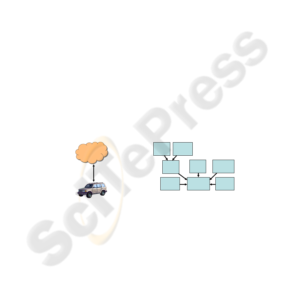
3 System Overview

Our system combines web and in-vehicle components to assist the driver in minimizing

their fuel purchase costs, as seen in Figure 1. To use the system, a driver must ﬁrst reg-

ister on a web portal and enter their fuel purchase preferences, such as how many times

per week they are willing to stop for gas and which brands they prefer. The web site

also assists the driver in mapping out their frequently traveled routes. The driver then

creates an approximate travel plan for the next week, which the system uses to identify

potential refueling stations. Future versions of our system will predict the driver’s future

driving routes without any input from the driver

Web server

Fig.1. System consisting of web to vehicle con-

nection.

Current

price

Historical

prices

User

preferences

Predicted

prices

Refueling

optimization

Vehicle

route

Wholesale

prices

Current

fuel level

Fig.2. This ﬁgure illustrates the data

ﬂow used in the refueling strategy op-

timization algorithm.

To get the most out of our system, the driver’s vehicle should include a navigation

system and a means of connecting the vehicle to the internet, such as a telematics plat-

form (e.g., OnStar [18], BMW Assist [1]) or a cell phone with data service (e.g. GPRS

or EVDO). The vehicle maintains a connection to the web server and periodically up-

loads the vehicle’s current fuel level and GPS location. An optimization algorithm (see

Section 5.1) on the web server uses the fuel level to calculate when and where the driver

should refuel and how many gallons to purchase. If the algorithm determines that the

driver should stop, it sends this information to the vehicle’s navigation system and alerts

the driver.

Figure 2 shows the main data sources our system uses to calculate a refueling plan.

Future fuel prices for individual fueling stations are predicted using a forecasting al-

gorithm (see Section 4) that takes into account historical prices as well as wholesale

prices. Historical and current prices are obtained from a database maintained by OPIS.

User preferences and vehicle routes are obtained from the web portal, and the current

fuel level is directly obtained from the vehicle.

4 Forecasting Model

As previously mentioned, if the consumer had more information on gasoline prices at

each gas station along the speciﬁed route and predicted prices for the next few days,

determining a refueling plan that would minimize the total fuel cost over the trip would

be achievable. One important aspect in determining the consumer’s refueling strategy

is an econometrical model that reasonably predicts daily gasoline retail prices at each

station on the route. Many studies show that the retail gasoline price is highly correlated

with wholesale gasoline price, according to the production and distribution system of

gasoline in the U.S [2]; this provides the foundation for our approach.

We present a simple forecasting approach that predicts future retail gas prices at

individual stations when the following limited data is available: wholesale regional gas

prices, one-month future market wholesale prices, current station retail gas prices, and

historical retail station gas prices. To determine which wholesale price to use as the

explanatory variable in our forecasting model, we considered several wholesale prices

to see which provided the best correlation to retail gas prices. There are four regional

wholesale prices in the U.S.: mid-continent, Los Angeles, New York, and Gulf coast

markets. These four regions and the one-month future market wholesale prices have

the following correlation with retail prices at gasoline stations in Michigan: 0.89, -0.71,

-0.89, 0.92, and -0.91, respectively. In addition, we tested the correlations between the

average of two or more wholesale prices and the retail gasoline prices: all values were

less than 0.92. As a result, we chose the Gulf coast wholesale price as our explanatory

variables in the model, which yielded the best correlation to retail gas prices.

The Energy Information Administration (EIA) reported in 1999 [5] that the down-

stream gasoline price responses caused by upstream price changes can be represented

by the following equation:

= β

(β

t−i

) + ε. (1)

Here D

is the price offered to each gas station by the supplier at time t; it is a moving

average of the wholesale prices U

t−i

at time t for the previous days i such that i =

1, . . . , 6. The error term is ε, which also represents the downstream markup.

The markup of each gasoline station π

at time t is the retail gasoline price p

time t at each gasoline station minus the price D

paid to its suppliers; that is,

= p

− D

. (2)

In this study, we do not use the coefﬁcients β provided by the EIA report, but esti-

mate coefﬁcients β by applying an Ordinary Least Square (OLS) linear regression [12]:

the retail gasoline price at time t is the dependent variable, and explanatory variables are

the wholesale prices U

t−i

for i = 1, . . . , 6, and the monthly dummy prices, M

, where

k = 1, . . . , 12 represents January through December, respectively, for any day t. The

results of this OLS linear regression are in Table 1. Applying the regression coefﬁcients,

β and θ, we can obtain the estimated suppliers’ prices D

= β

(β

t−i

) +

(θ

). (3)

Table 1. Relationship between retail gas and mid-continent wholesale prices: R

= 0.97, ***Sta-

tistically signiﬁcant at 99% conﬁdence level, *Statistically signiﬁcant at 90% conﬁdence level.

Variable Coefﬁcient (β) Standard Error

t−1

0.002 *** 0.001

t−2

0.001 0.001

t−3

0.001 0.001

t−4

0.001 0.001

t−5

4.531 e-04 0.001

t−6

0.003*** 0.001

-0.180 *** 0.014

-0.090*** 0.020

-0.039* 0.031

0.020 0.038

0.089*** 0.033

0.088*** 0.032

0.102 *** 0.025

-0.012 0.030

0.001 0.041

0.009* 0.006

constant 0.950*** 0.059

So, the estimated markup of each gasoline station at time t is π

= p

− D

. How-

ever, we randomly chose some gasoline stations to study their markup and found some

interesting markup patterns. For each day of the week, even if the markup π

is dif-

ferent for every t, it is always higher at the end of a week and lower at the beginning

of a week. Since it is not feasible to test each gasoline station’s markup, we make the

assumption from our comprehensive testing that gasoline prices at each gasoline station

have a weekly pattern; without loss of generalization, we calculate the average markup

for each weekday, providing us with seven average markups for each gasoline station.

We call this average markup for each weekday ˜π

for n = 1, . . . , 7; i.e. for each day

of the week n, we calculate the average markup for n using historical data for n. For

example, to calculate ˜π

for n = 1 (Monday), we take the average markup over all

Mondays (π

such that t is a Monday) in our historical data. Hence, we can predict the

gas price for any station one day in advance by

t+1

= D

t+1

+ ˜π

, (4)

where n = 1, . . . , 7 represents Monday through Sunday, respectively, for any day t.

When retail gas price for time t is not available for a speciﬁc station, we can also use

equation (4) to estimate the missing price.

To forecast the gasoline prices at one speciﬁc gasoline station more than one day

in advance, we can do so using p

t+i

= D

t+1

+ ˜π

n+i

, for i = 1 to m, where m is the

number of days ahead for which the forecast is desired. Because we do not know the

wholesale or suppliers’ prices on days t+i, when i > 1, the accuracy of the forecasting

results will decrease as i increases.

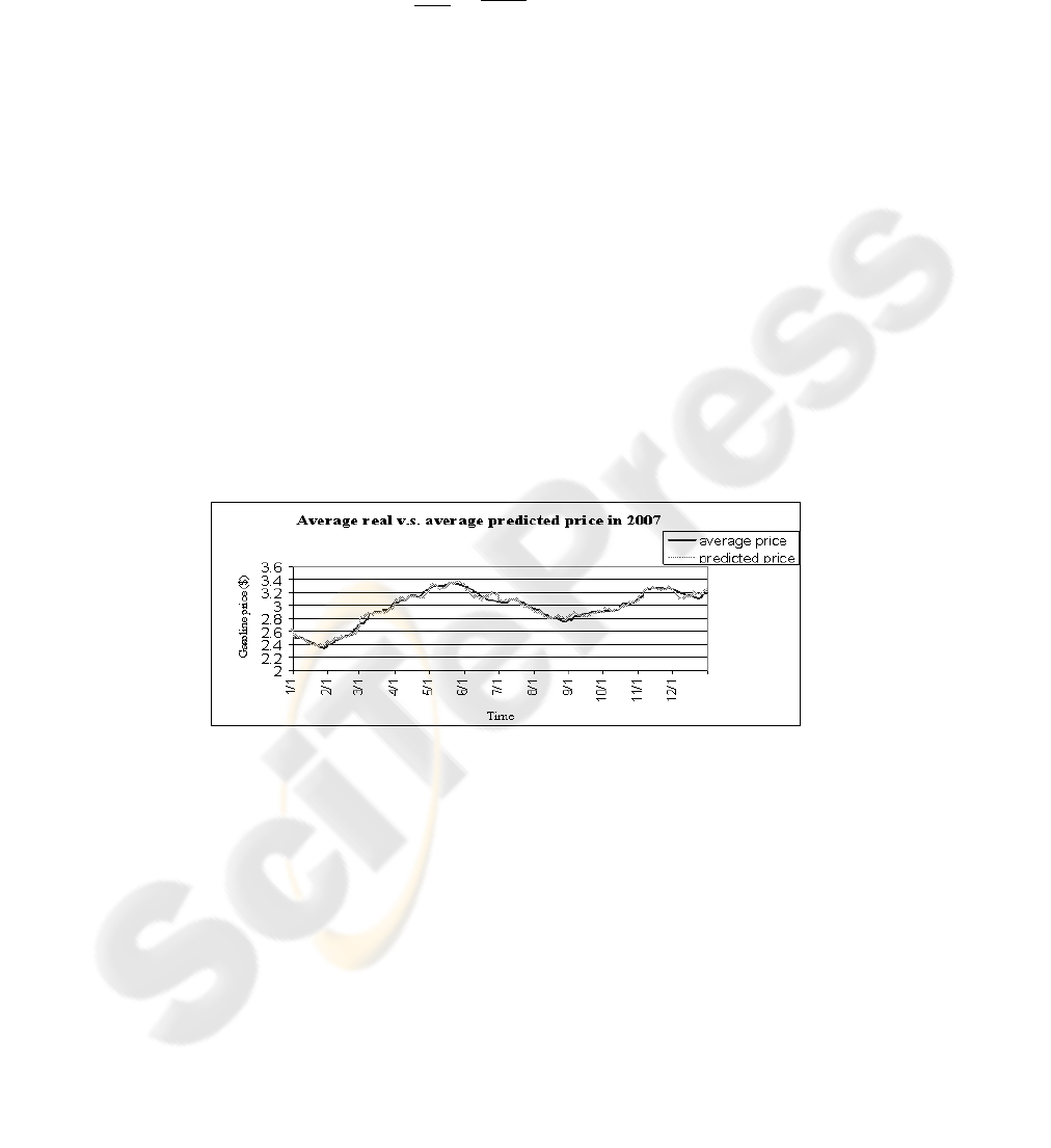
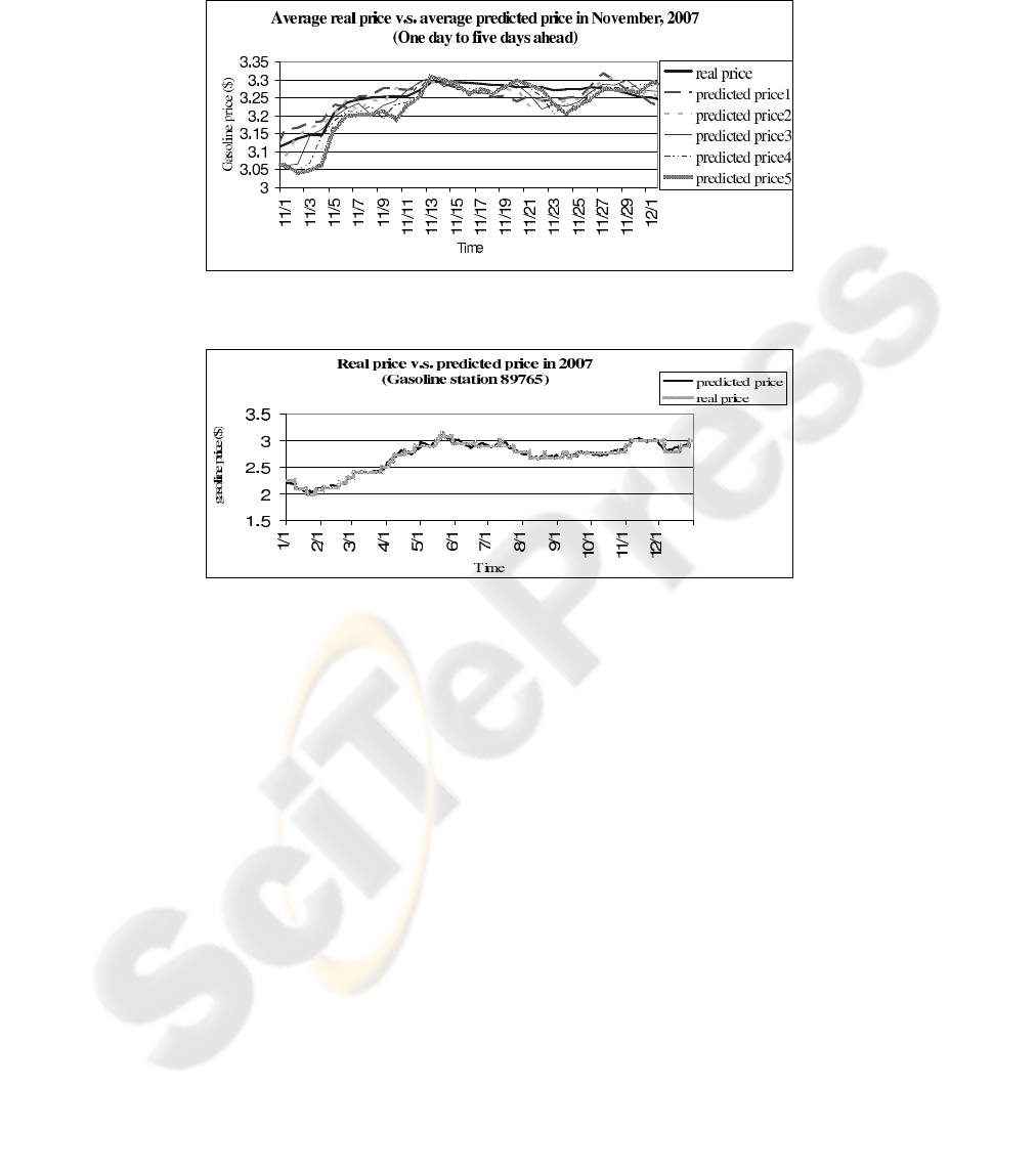
The graphs below show the prediction results from the simple price forecasting

model described above for gas purchases using 2007 daily data. Figure 3 and 4 dis-

play average daily retail gasoline prices (averages include prices for 931 stations) and

predicted gasoline prices in Michigan. Figure 3 shows the average daily retail gasoline

prices compared to the predicted gasoline prices based on the one-day ahead predic-

tion for Michigan over 2007. Figure 4 includes ﬁve predicted prices which are one-day

ahead, two-day ahead, three-day ahead, four-day ahead and ﬁve-day ahead, respectively,

for the month of November 2007. For example, when using the three-day ahead predic-

tions, we would use November 1, 2007 data to predict the price of gas on November 4,

2007. The mean of absolute residual values (i.e., the absolute difference between real

price and predicted price) for the one to ﬁve day ahead predictions are approximately

3.2 cents, 2.8 cents, 2.9 cents, 3.1 cents, and 3.3 cents; the standard deviation of the

absolute residual values is 2.3 cents, 2 cents, 2.1 cents, 2.2 cents and 2.4 cents, respec-

tively. Figure 5 show the predicted daily gasoline prices at one stations in Michigan as

an example to demonstrate the accuracy of predicted prices for an individual gas station.

Fig.3. Average retail price compared to average predicted retail price for 931 gasoline stations.

Some papers discuss factors that impact daily or weekly gasoline price ﬂuctuation

[4], but few researchers have studied forecasting models for daily gasoline prices. Com-

pared to those models, our approach for price prediction provides a simple way when

limited data is available to estimate daily gasoline price at each gasoline station with

forecasting results that are within a reasonable range to the retail prices. In future re-

search, we plan to develop a more advanced forecasting model that will require more

data, but will be able to include effects of other factors on retail gasoline prices, such

as a gasoline station’s brand, distance to competitors, station characteristics, regional

income level, etc. Moreover, we will use an autoregressive integrated moving average

(ARIMA) model [12] to better understand the lag terms t−i (the number of days before

t that are considered) and their coefﬁcients.

Fig.4. Average retail price and 5 average predicted prices of 931 stations in November, 2007.

Fig.5. Real retail price and predicted retail price at gasoline station 89765 in 2007

5 Solution Techniques

Once we have the forecasted gas prices, we are ready to use these as cost inputs to

the objective function in our optimization model. There are a number of different ap-

proaches for solving the optimal refueling strategy problem from heuristical approaches

to discrete optimization methods. In this paper, we ﬁrst describe how to model the re-

fueling strategy optimization problem as a Mixed Integer Program (MIP) [21]. Next,

we brieﬂy explore two simple heuristics: the ﬁrst has the driver stop at the cheapest gas

station in the area whenever the driver runs out of gas, and the second recommends a

refueling stop within a certain tank capacity range.

5.1 Mixed Integer Program

We ﬁrst describe the MIP optimization technique, introducing the input information,

discussing the variables, the objective function, and ending with a detailed description

of the constraints and overall model formulation.

Input Information. In this section, we describe the parameters that are inputs to the

MIP model. We divide these inputs into the following categories: inputs obtained from

vehicle internal network, inputs implicit from route speciﬁcations, inputs deﬁned by

user to specify preferences, and inputs from the forecasting model. We deﬁne a route to

be a multi-day trip plan of around one week. After a week, the accuracy of the forecasted

gas prices diminishes. However, the week can be a rolling horizon, where the model is

solved every day for a new week time period.

We get the following information from the vehicle internal network:

Max = maximum number of gallons the gas tank holds

MPG = miles per gallon (note that this could be different depending on the route)

= initial amount of gas in the vehicle at the beginning of the route

As discussed in Section 3, driver routes are continually being collected on the vehicle

internal network to populate the user’s most frequently driven routes or can be set up

on the web portal by the driver for routes not previously driven.

Knowing these routes, we can determine the following inputs:

n = number of gas stations in route

S = set of gas stations in route = {1, 2, . . . , n}

m = number of driving days or time periods in the route

D = set of days = {1, 2, . . . , m}

= the distance from the starting point of the route to gas station i

= the distance from each station i back to the original route

NP I

= the new period index ∀ t ∈ D. The gas stations are sorted in the order in

which the driver will encounter them along the route. NP I

identiﬁes the

ﬁrst gas station encountered on day t. For example, N P I

= 1 is the index

for the ﬁrst gas station in the ﬁrst time period. If on the second day (t = 2)

the ﬁrst gas station to visit is station 256, then NP I

= 256.

In addition to the routes, the user speciﬁes the following preferences through the

web portal:

Min = minimum number of gallons of gas the driver wants to have in the fuel tank

at any given time

MST = maximum number of stops over the entire route (note that this

should take into consideration the number of miles driven so that the

problem does not become infeasible)

MSD = maximum number of stops in one day of the trip (note that this

should take into consideration the number of miles driven so that the

problem does not become infeasible)

The last input involves the cost of gas at each station. If the gas station occurs along

the route on the current day, then the cost of gas is the current gas price. If the gas

station occurs along the route on a future day or the current day’s price is not available,

then it comes from the forecasting model.

= cost of gas at station i.

We keep track of the ﬁrst station in each time period, so we get the corresponding

forecasted gas prices p

t+i−1

for days i = 2, . . . , m for each station.

Variables. This model contains both binary and continuous variables. The binary vari-

ables help make choices of when to stop, whereas the continuous variables determine

how much gas to get at a station.

– The ﬁrst variable, x

, is a binary variable that determines whether or not the driver

should stop at gas station i. In other words,

1 if stop at gas station i

0 otherwise

∀i ∈ S.

Recall that the time period is embedded in this variable as we keep track of it by

the value NP I

– The second variable, y

, is the amount (in gallons) of gas purchased from station i

for every i ∈ S.

Objective Function. The objective is to minimize the total amount spent on gas when

traveling on a speciﬁc route over a certain number of days. The user preferences of how

many times they are willing to stop also comes into play by adding a weighted penalty

to the number of stops. If the user does not set a preference for the number of stops, then

we let α = 0; that is, we don’t impose a penalty. The objective function is as follows

min

+ αx

) (5)

Constraints. In this section, we will discuss the constraints that are involved in guar-

anteeing that the driver does not run out of gas, that the driver does not get more gas

than the fuel tank can hold, and if the driver stops at a station than the driver must get

gas.

The ﬁrst constraint speciﬁes that the vehicle must never run out of gas. So, when the

vehicle gets to station i, the amount of gas that the vehicle had at station i −1 needs to

be enough to get to station i and still have the minimum gallons required. Note that we

add the distance ξ

to account for the distance that the driver takes if they stop at some

station j < i to get back to their route.

Min ≤ G

−

MP G

j<i

−

j<i

MP G

∀ i ∈ S. (6)

The second constraint guarantees that the vehicle will never have more gas than the

amount held by the fuel tank. So, for every station visited,

−

MP G

j≤i

−

j<i

MP G

≤ Max ∀ i ∈ S. (7)

We also constrain the number of stops per route; this accounts for how much gas the

vehicle’s tank can hold so that the problem does not become infeasible.

i∈S

≤ M ST (8)

Or, if we only want a maximum number of stops per day, we address it by the

following two constraints. The ﬁrst constraint is for all time periods except for the last

one, and the second constraint covers the last time period:

i∈S:i≥NP I

t−1

&i<NP I

≤ M SD ∀ t ∈ D \1,

i∈S:i≥NP I

&i≤n

≤ M SD. (9)

The last two constraints are linking constraints that guarantee if the driver does not

stop at station i to get gas then no gallons should be purchased; that is,

≤ (Max −Min)x

∀ i ∈ S and x

≤ y

∀ i ∈ S. (10)

Bounds. The variable x

is a binary variable. The variable y

is a real number that must

be greater than or equal to zero, but less than or equal to the size of the fuel tank minus

the preference of how much fuel should always be left in the tank. Note that the upper

bound on the y

variable is implied by the ﬁrst linking constraint in (10). The bounds

are as follows: x

∈ B ∀ i ∈ S and 0 ≤ y

≤ Max −Min such that y

∈ < ∀ i ∈ S.

Problem Formulation.

min

, y

∀i ∈ S

+ αx

)

s.t.

Min ≤ G

−

MP G

j<i

−

j<i

MP G

∀ i ∈ S

−

MP G

j≤i

−

j<i

MP G

≤ Max ∀ i ∈ S

i∈S

≤ M ST

i∈S:i≥NP I

t−1

&i<NP I

≤ M SD ∀ t ∈ D \ 1

i∈S:i≥NP I

&i≤n

≤ M SD

≤ (Max −Min)x

∀ i ∈ S and x

≤ y

∀ i ∈ S

∈ B ∀ i ∈ S and 0 ≤ y

≤ Max −Min

5.2 Heuristics

Two different heuristic approaches are considered as possible solution techniques. The

ﬁrst approach has the driver stop for gas whenever the fuel gage hits a minimum allow-

able fuel level. For example, if this minimum level is 2 gallons then the driver will stop

at the gas station right before the fuel level drops to 2 gallons. When stoping for gas

the driver always refuels to the maximum tank capacity. This method may not give the

lowest total fuel cost over a trip, however it will result in the minimum number of stops

possible to complete the trip. The second method is a Greedy heuristic where the driver

continues along their given route until the fuel gage registers a predetermined amount.

As an example, let this predetermined amount be half a tank of gas. At this point, the

heuristic checks all of the given gas stations between half a tank and the minimum al-

lowable fuel level. The station with the lowest gas price in this range is selected as the

refueling point, and when the driver stops, they ﬁll their tank to the maximum capac-

ity. The driver then continues along the route until the fuel level reaches half a tank,

at which point the process repeats itself. This method should show some improvement

in fuel costs compared with the previous heuristic and will eliminate the possibility of

purchasing small amounts of gas at any given stop.

6 Example Scenario

A sample scenario was created to demonstrate the various solution techniques and to

compare resulting MIP solutions when user preferences are considered. In this scenario,

a ﬁve day trip has been planned in which there are 1532 possible gas stations to stop at

along the route. For each gas station, the forecasted price of gas and the distance from

the starting point is known. The driver’s vehicle averages 22 miles per gallon, holds a

maximum 15 gallons of gas, and is starting the trip with 5 gallons of fuel. The driver

preferences are not to let the fuel level drop below 2 gallons and no stopping for gas

more than twice in one day or more than six times over the entire trip.

Table 2. Scenario Results for Optimization Methods.

Optimization Optimization with Penalty

Day ID Distance Price ($) Buy Day ID Distance Price ($) Buy

1 28 15.571 2.799 10.708 1 41 26.685 2.799 11.213

1 171 115.498 2.799 4.542 2 367 284.007 2.837 10.544

3 484 373.707 2.821 6.507 4 853 544.649 2.719 8.098

4 853 544.649 2.719 8.098 5 1240 722.803 2.698 7.539

5 1240 722.803 2.698 7.539 N/A

Total Trip Fuel Cost: $ 103.398 Total Trip Fuel Cost: $ 103.655

Table 2 displays the following results for the scenario: a listing of on which days

to stop, at which gas stations to stop, the price of gas at each station, and how much

gas should be purchased at each station. The ﬁrst column (Optimization) provides the

solution when the objective function is to minimize to cost of fuel over the trip and α

is set to zero such that there is no penalty for the number of stops. The second col-

umn (Optimization with Penalty) provides the results for the optimization model that

includes a penalty in the objective function each time the driver has to stop for gas;

this enforces user preferences on how many times a day and per trip they are willing

to stop (see equation 5). Here we set α = 1, but the value of α could vary depending

on the number of gas stations considered in the route. If we compare the results for the

optimization models with different objective functions, we see the difference caused by

the penalty in the objective function: it eliminates an additional stop on the ﬁrst day for

a slight increase in overall cost of around $.25.

Table 3 shows the results for both heuristic methods when applied to this scenario.

The ﬁrst column gives the solution when the driver stops for gas right before their fuel

gage registers the minimum gas allowed (2 gallons in this scenario). The second column

gives the results of the greedy heuristic, which looks for the lowest priced gas between

when the fuel gage registers half a tank and 2 gallons.

Table 4 compares the results of the four approaches. The heuristic, which has the

driver stop at the closest gas station when they reach 2 gallons of gas in their tank, results

in the fewest stops and eliminates only partially ﬁlling up the gas tank when stoping.

However, this technique does result in the highest total fuel cost which is 6.44% higher

than the original optimization technique.

Table 3. Scenario Results for Heuristic Methods.

Stop At 2 Gallons Greedy Heuristic

Day ID Distance Price ($) Buy Day ID Distance Price ($) Buy

1 101 65.892 2.999 12.995 1 41 26.685 2.799 11.213

2 432 350.930 2.946 12.956 2 381 290.172 2.837 11.977

4 1061 636.879 2.877 11.442 4 924 563.492 2.719 12.424

N/A 5 1446 829.094 2.698 1.78

Total Trip Fuel Cost: $ 110.06 Total Trip Fuel Cost: $ 103.945

Table 4. Technique Comparison.

Optimization Optimization with Penalty Stop at 2 Gallons Greedy

# Stops 5 4 3 4

Stops Fill < 10 Gallons 4 2 0 1

Total Cost ($) 103.398 103.655 110.06 103.945

% Over Lowest Cost N/A 0.25% 6.44% 0.53%

7 Conclusions

With fuel prices on the rise in the United States, drivers are increasingly concerned with

their refueling strategy. This paper presented a model to assist drivers with decisions

regarding where and when to refuel along with how much fuel to purchase. The model

takes into account various factors, such as user preferences (e.g. how often the driver

is willing to stop for gas) and vehicle speciﬁc information (e.g. the current fuel level).

Gas stations along a speciﬁed route can be identiﬁed and gas prices corresponding to

future days of the route can be determined using the forecasting method discussed in

Section 4. Once this information has been aggregated, it is used by the Mixed Integer

Programming model presented in Section 5.1 to provide the driver with an optimal

refueling strategy. As shown in section 5.2 heuristical approaches can also be used to

determine a refueling strategy.

Future versions of this model can be extended to include additional driver prefer-

ences or economic factors. For example, by considering ﬂex-fuel vehicles, the refueling

decision becomes even more complex as the analysis would include tradeoffs between

the price per gallon of fuel, average miles per gallon associated with a particular route

and vehicle, and possibly the CO2 effects for multiple fuel types. In addition, we could

move towards a more advanced forecasting model and provide a refueling strategy that

would take into consideration multiple routes for a single origin destination pair.

The proposed model offers substantial beneﬁts over existing approaches. First, it

provides an optimal refueling strategy using forecasted fuel prices over multiple time

periods and locations as opposed to a local strategy based on a small geographical

region and the current fuel prices in that area. In addition, the vehicle internal network

can be used to monitor the current fuel level and consumption to offer proactive advice

instead of waiting for the driver to request help from the system. Finally, over time the

system can learn a driver’s regular routes and associated fuel consumption to provide

more accurate recommendations in the proposed refueling strategy.

Acknowledgements

We would like to thank Jenny Lin at Corporate Economics of Ford Motor Company for

providing the 5 series of wholesale prices.

References

1. BMW. BMW website. http://www.bmwusa.com/Standard/Content/Owner/

BMWAssist/Default.aspx, 2008.

2. Borenstein, Cameron & Gilbert. Do gasoline prices respond asymmetrically to crude oil

price changes? TheQuarterlyJournalofEconomics,Vol.112,1997, 1999.

3. Dash. Dash website. http://www.dash.net/, 2008.

4. Eckert, & West. Retail gasoline price cycles across spatially dispersed gasoline stations.

JournalofLawandEconomics,April,2004, 2004.

5. Energy Information Administration. Price changes in the gasoline market. http://

tonto.eia.doe.gov/FTPROOT/petroleum/0626.pdf, 1997.

6. Farecast. Our Technology and Data website, 2008. http://www.farecast.com/

about/ourTechnology.do.

7. Ford Motor Company. Popular Ford SYNC System Expanded; New SIRIUS ”Travel Link”

Takes Navigation to New Level website, 2008. http://media.ford.com/article_

display.cfm\?article_id=27489.

8. J. Froehlich and J. Krumm. Route predictions from trip observations. Society of Automotive

Engineers (SAE) 2008 World Congress, April 2008.

9. Garmin. https://buy.garmin.com/shop/shop.do?pID=13479, 2008.

10. GasBuddy. GasBuddy website. http://www.gasbuddy.com/, 2008.

11. GasPriceWatch. GasPriceWatch website. http://www.gaspricewatch.com/, 2008.

12. William Greene. Econometric Analysis. Prentice Hall, 2007.

13. E. Horvitz, P. Koch, and M. Subramani. Mobile Opportunistic Planning: Methods and Mod-

els, pages 228–237. Lecture Notes in Computer Science. Springer Berlin, 2007.

14. Integrated Decision Support. Planning and Execution Solutions for Truckload Carriers: Ex-

pert Fuel website, 2008. http://www.idscnet.com/software/fuel.htm.

15. E. Kamar, E. Horvitz, and C. Meek. Mobile opportunistic commerce: Mechanisms, archi-

tecture, and application. In Proceedings of AAMAS 2008, Estoril, Portugal, May 2008.

16. A. Kapoor and E. Horvitz. Experience sampling for building predictive user models: A

comparative study. In Proceedings of CHI 2008, Florence, Italy, April 2008.

17. Ludovic Privat. TomTom to offer real-time fuel price to GO 920. GPS Business News,

January 10 2008.

18. OnStar. OnStar website. http://www.onstar.com/, 2008.

19. OPIS. OPIS website. http://www.opisnet.com/, 2008.

20. The Gas Game. The Gas Game website. http://www.thegasgame.com/, 2008.

21. L. Wolsey. Integer Programming. John Wiley & Sons, Inc., 1998.