THE BEES ALGORITHM
AND MECHANICAL DESIGN OPTIMISATION
D. T. Pham, M. Castellani, M. Sholedolu
Manufacturing Engineering Centre, Cardiff University, Cardiff, U.K.
A. Ghanbarzadeh
Mechanical Engineering Department, Engineering Faculty, Shahid Chamran University, Ahvaz, Iran
Keywords: Bees Algorithm, Optimisation, Mechanical Design.
Abstract: The Bees Algorithm is a search procedure inspired by the way honey-bees forage for food. A standard
mechanical design problem, the design of a welded beam structure, was used to benchmark the Bees
Algorithm against other optimisation techniques. The paper presents the results obtained showing the robust
performance of the Bees Algorithm.
1 INTRODUCTION
Researchers have used the design of welded beam
structures (Rekliatis et al., 1983) as a benchmark
problem to test their optimisation algorithms. The
welded beam design problem involves a nonlinear
objective function and eight constraints. A number
of optimisation techniques have been applied to this
problem. Some of them, such as geometric
programming (Ragsdell and Phillips, 1976), require
extensive problem formulation; some (see, for
example, (Leite and Topping, 1998)) use specific
domain knowledge which may not be available for
other problems, and others (see, for example,
(Ragsdell and Phillips, 1976)) are computationally
expensive or give poor results.
The Bees Algorithm has been applied to
different optimisation problems (Pham et al., 2005,
Pham et al., 2006b, Pham et al., 2006a). The design
problems discussed in this paper are constrained
optimisation problems to be solved using this new
algorithm.
The remainder of the paper is structured as
follows. Section 2 explains the main features of the
foraging process and the steps of the Bees
Algorithm. Section 3 describes the welded beam
design problem. Section 4 presents the results
obtained using the Bees Algorithm and other
optimisation procedures. Section 5 concludes the
paper.
2 THE BEES ALGORITHM
2.1 The Foraging Process in Nature
During the harvesting season, a colony of bees keeps
a percentage of its population as scouts (Von Frisch,
1976) and uses them to explore the field surrounding
the hive for promising flower patches. The foraging
process begins with the scout bees being sent to the
field where they move randomly from one patch to
another.
When they return to the hive, those scout bees
that found a patch of a sufficient quality (measured
as the level of some constituents, such as sugar
content) deposit their nectar or pollen and go to the
“dance floor” to perform a dance known as the
“waggle dance” (Seeley, 1996). This dance is the
means to communicate to other bees three pieces of
information regarding a flower patch: the direction
in which it will be found, its distance from the hive,
and its quality rating (or fitness) (Von Frisch, 1976,
Camazine et al., 2003). This information helps the
bees watching the dance to find the flower patches
without using guides or maps. After the waggle
dance, the dancer (i.e. the scout bee) goes back to
250
T. Pham D., Castellani M., Sholedolu M. and Ghanbarzadeh A. (2008).
THE BEES ALGORITHM AND MECHANICAL DESIGN OPTIMISATION.
In Proceedings of the Fifth International Conference on Informatics in Control, Automation and Robotics - ICSO, pages 250-255
DOI: 10.5220/0001506102500255
Copyright
c
 SciTePress

the flower patch with follower bees recruited from
the hive. The number of follower bees will depend
on the overall quality of the patch. Flower patches
with large amounts of nectar or pollen that can be
collected with less effort are regarded as more
promising and attract more bees (Seeley, 1996,
Bonabeau et al., 1999). In this way, the colony can
gather food quickly and efficiently.
2.2 The Bees Algorithm
This section summarises the main steps of the Bees
Algorithm. For more details, the reader is referred to
(Pham et al., 2006b, Pham et al., 2006a, Pham et al.,
2005). Figure 1 shows the pseudo code for the Bees
Algorithm. The algorithm requires a number of
parameters to be set, namely: number of scout bees
(n), number of sites selected for neighbourhood
searching (out of n visited sites) (m), number of top-
rated (elite) sites among m selected sites (e), number
of bees recruited for the best e sites (nep), number of
bees recruited for the other (m-e) selected sites
(nsp), the initial size of each patch (ngh) (a patch is a
region in the search space that includes the visited
site and its neighbourhood), and the stopping
criterion. The algorithm starts with the n scout bees
being placed randomly in the search space. The
fitnesses of the sites visited by the scout bees are
evaluated in step 2.
1. Initialise population with random
solutions.
2. Evaluate fitness of the population.
3. While (stopping criterion not met)
//Forming new population.
4. Select sites for neighbourhood search.
5. Determine the patch size.
6. Recruit bees for selected sites (more
bees for best
e sites) and evaluate
fitnesses.
7. Select the fittest bee from each patch.
8. Abandon sites without new
information.
9. Assign remaining bees to search
randomly and evaluate their fitnesses.
10. End While.
Figure 1: Pseudo code of the Bees Algorithm.
In step 4, the m sites with the highest fitnesses
are designated as “selected sites” and chosen for
neighbourhood search. In step 5, the size of
neighbourhood around the selected sites is
determined. In step 6, the algorithm conducts
searches around the selected sites, assigning more
bees to search in the vicinity of the best e sites.
Selection of the best sites can be made directly
according to the fitnesses associated with them.
Alternatively, the fitness values are used to
determine the probability of the sites being selected.
Searches in the neighbourhood of the best e sites –
those which represent the most promising solutions -
are made more detailed. As already mentioned, this
is done by recruiting more bees for the best e sites
than for the other selected sites. Together with
scouting, this differential recruitment is a key
operation of the Bees Algorithm.
In step 7, for each patch, only the bee that has
found the site with the highest fitness (the “fittest”
bee in the patch) will be selected to form part of the
next bee population. In nature, there is no such a
restriction. This restriction is introduced here to
reduce the number of points to be explored. In step
8, sites which have not shown improvements in
fitness values over a number of recruitment cycles
are abandoned. This is because it is assumed that
such sites correspond to stationary points. The
locations of the sites are recorded. In step 9, the
remaining bees in the population are assigned
randomly around the search space to scout for new
potential solutions.
At the end of each iteration, the colony will have
two parts to its new population: representatives from
the selected patches, and scout bees assigned to
conduct random searches. These steps are repeated
until a stopping criterion is met.
As described above, the Bees Algorithm is
suitable for unconstrained optimisation problems. If
a problem involves constraints, a simple technique
can be adopted to enable the optimisation to be
applied. The technique involves subtracting a large
number from the fitness of a particular solution that
has violated a constraint in order drastically to
reduce the chance of that solution being found
acceptable. This was the technique adopted in this
work. As both design problems were minimisation
problems, a fixed penalty was added to the cost of
any constraint-violating potential solution.
THE BEES ALGORITHM AND MECHANICAL DESIGN OPTIMISATION
251

3 WELDED BEAM DESIGN
PROBLEM
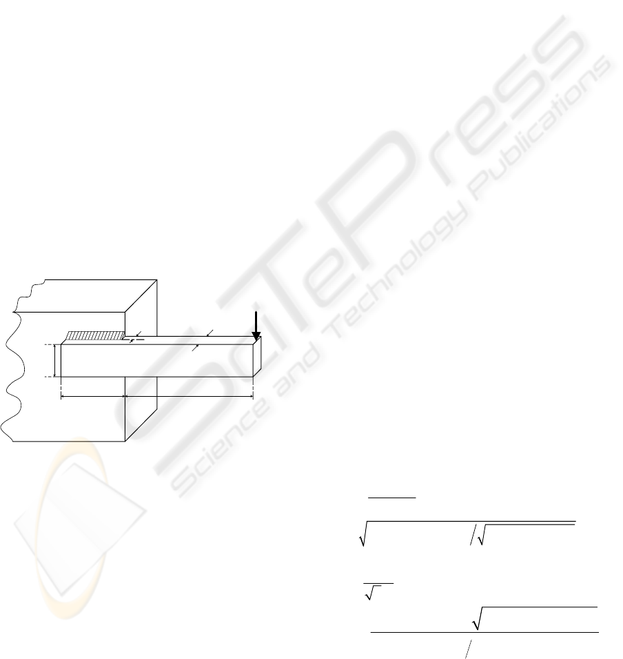
A uniform beam of rectangular cross section needs
to be welded to a base to be able to carry a load of
6000 lbf
. The configuration is shown in Figure 2.
The beam is made of steel 1010.
The length L is specified as 14 in. The objective
of the design is to minimise the cost of fabrication
while finding a feasible combination of weld
thickness h, weld length l, beam thickness t and
beam width b. The objective function can be
formulated as (Rekliatis et al., 1983) :
Min
2
12
(1 ) ( )
f
chl ctbL l=+ + + (1)
where
f
= Cost function including setup cost, welding
labour cost and material cost;
1
c = Unit volume of weld material cost
=
3
0.10471 $ / .in
;
2
c = Unit volume of bar stock cost
=
3
0.04811 $ / .in
;
L = Fixed distance from load to support =
14 in
;
Figure 2: A Welded Beam.
Not all combinations of h, l, t and b which can
support F are acceptable. There are limitations
which should be considered regarding the
mechanical properties of the weld and bar, for
example, shear and normal stresses, physical
constraints (no length less than zero) and maximum
deflection. The constraints are as follows (Rekliatis
et al., 1983):
1
0
d
g ττ =−≥ (2)
2
0
d
g σσ =−≥
(3)
3
0gbh=−≥
(4)
4
0gl=≥
(5)
5
0gt=≥ (6)
6
0
c
gPF=−≥ (7)
7
0.125 0gh=− ≥ (8)
8
0.25 0g δ =−≥ (9)
where
d
τ = Allowable shear stress of weld =
13600
P
si
;
τ = Maximum shear stress in weld;
d
σ = Allowable normal stress for beam material
=
30000
P
si
;
σ = Maximum normal stress in beam;
c
P = Bar buckling load;
F
= Load =
6000 lbf
;
δ = Beam end deflection.
The first constraint (
1
g ) ensures that the
maximum developed shear stress is less than the
allowable shear stress of the weld material. The
second constraint (
2
g ) checks that the maximum
developed normal stress is lower than the allowed
normal stress in the beam. The third constraint (
3
g )
ensures that the beam thickness exceeds that of the
weld. The fourth and fifth constraints (
4
g and
5
g
)
are practical checks to prevent negative lengths or
thicknesses. The sixth constraint (
6
g ) makes sure
that the load on the beam is not greater than the
allowable buckling load. The seventh constraint
(
7
g ) checks that the weld thickness is above a given
minimum, and the last constraint (
8
g ) is to ensure
that the end deflection of the beam is less than a
predefined amount.
Normal and shear stresses and buckling force
can be formulated as (Shigley, 1973, Rekliatis et al.,
1983):
3
2.1952
tb
σ =
(10)
22 2 2
() () ( ) 0.25( ( ))llht ττ τ ττ
′′′ ′′′
=++ ++
(11)
where
6000
2hl
τ
′
=
(Primary stress)
()
()
{}
22
2
2
6000(14 0.5 ) 0.25( ( ) )
2 0.707 12 0.25
llht
hl l h t
τ
+++
′′
=
++
(Secondary stress)
B
A
F
h
b
t
l
L
ICINCO 2008 - International Conference on Informatics in Control, Automation and Robotics
252

3
64746.022(1 0.0282346 )
c
Pttb=−
(12)
4 RESULTS AND DISCUSSION
The empirically chosen parameters for the Bees
Algorithm are given in Table 1 with the stopping
criterion of 750 generations. The search space was
defined by the following intervals (Deb, 1991):
0.125 5h≤≤ (13)
0.1 10l≤≤ (14)
0.1 10t≤≤ (15)
0.1 5b≤≤ (16)
With the above search space definition,
constraints
4
g ,
5
g and
7
g are already satisfied and
do not need to be checked in the code.
Table 1: Parameters of the Bees Algorithm for the welded
beam design problem.
Bees Algorithm parameters Symbol Value
Population n 80
Number of selected sites m 5
Number of top-rated sites out
of m selected sites
e 2
Initial patch size ngh 0.1
Number of bees recruited for
best e sites
nep 50
Number of bees recruited for
the other (m-e) selected sites
nsp 10
Figure 3: Evolution of the lowest cost in each iteration.
Figure 3 shows how the lowest value of the
objective function changes with the number of
iterations (generations) for three independent runs of
the algorithm. It can be seen that the objective
function decreases rapidly in the early iterations and
then gradually converges to the optimum value.
A variety of optimisation methods have been
applied to this problem by other researchers
(Ragsdell and Phillips, 1976, Deb, 1991, Leite and
Topping, 1998). The results they obtained along
with those of the Bees Algorithm are given in Table
2. APPROX is a method of successive linear
approximation (Siddall, 1972). DAVID is a gradient
method with a penalty (Siddall, 1972). Geometric
Programming (GP) is a method capable of solving
linear and nonlinear optimisation problems that are
formulated analytically (Ragsdell and Phillips,
1976). SIMPLEX is the Simplex algorithm for
solving linear programming problems (Siddall,
1972).
As shown in Table 2, the Bees Algorithm
produces better results than almost all the examined
algorithms including the Genetic Algorithm (GA)
(Deb, 1991), an improved version of the GA (Leite
and Topping, 1998), SIMPLEX (Ragsdell and
Phillips, 1976) and the random search procedure
RANDOM (Ragsdell and Phillips, 1976). Only
APPROX and DAVID (Ragsdell and Phillips, 1976)
produce results that match those of the Bees
Algorithm. However, as these two algorithms
require information specifically derived from the
problem (Leite and Topping, 1998), their application
is limited. The result for GP is close to those of the
Bees Algorithm but GP needs a very complex
formulation (Ragsdell and Phillips, 1976).
5 CONCLUSIONS
A constrained optimisation problem was solved
using the Bees Algorithm. The algorithm converged
to the optimum without becoming trapped at local
optima. The algorithm generally outperformed other
optimisation techniques in terms of the accuracy of
the results obtained. A drawback of the algorithm is
the number of parameters that must be chosen.
However, it is possible to set the values of those
parameters after only a few trials.
Indeed, the Bees Algorithm can solve a problem
without any special domain information, apart from
that needed to evaluate fitnesses. In this respect, the
Bees Algorithm shares the same advantage as global
search algorithms such as the Genetic Algorithm
(GA). Further work should be addressed at reducing
the number of parameters and incorporating better
learning mechanisms to make the algorithm even
simpler and more efficient.
0
2
4
6
8
10
0 1530456075
Gene ration x 10
-1
Cost
BA Run 1
BA Run 2
BA Run 3
Optimum
THE BEES ALGORITHM AND MECHANICAL DESIGN OPTIMISATION
253

Table 2: Results for the welded beam design problem obtained using the Bees Algorithm and other optimisation methods.
Methods
Design variables
Cost
h l t b
APPROX
(Ragsdell and
Phillips, 1976)
0.2444 6.2189 8.2915 0.2444 2.38
DAVID (Ragsdell
and Phillips,
1976)
0.2434 6.2552 8.2915 0.2444 2.38
GP (Ragsdell and
Phillips, 1976)
0.2455 6.1960 8.2730 0.2455 2.39
GA (Deb, 1991)
Three
independent
runs
0.2489 6.1730 8.1789 0.2533 2.43
0.2679 5.8123 7.8358 0.2724 2.49
0.2918 5.2141 7.8446 0.2918 2.59
IMPROVED GA
(Leite and
Topping, 1998)
Three
independent
runs
0.2489 6.1097 8.2484 0.2485 2.40
0.2441 6.2936 8.2290 0.2485 2.41
0.2537 6.0322 8.1517 0.2533 2.41
SIMPLEX
(Ragsdell and
Phillips, 1976)
0.2792 5.6256 7.7512 0.2796 2.53
RANDOM
(Ragsdell and
Phillips, 1976)
0.4575 4.7313 5.0853 0.6600 4.12
BEES
ALGORITHM
Three
independent
runs
0.24429 6.2126 8.3009 0.24432 2.3817
0.24428 6.2110 8.3026 0.24429 2.3816
0.24432 6.2152 8.2966 0.24435 2.3815
ACKNOWLEDGEMENTS
The research described in this paper was performed
as part of the Objective 1 SUPERMAN project, the
EPSRC Innovative Manufacturing Research Centre
Project and the EC FP6 Innovative Production
Machines and Systems (I*PROMS) Network of
Excellence.
REFERENCES
Bonabeau, E., Dorigo, M. & Theraulaz, G. (1999) Swarm
Intelligence: from Natural to Artificial Systems, New
York, Oxford University Press.
Camazine, S., Deneubourg, J.-L., Franks, N. R., Sneyd, J.,
Theraula, G. & Bonabeau, E. (2003) Self-Organization
in Biological Systems, Princeton, Princeton University
Press.
Deb, K. (1991) Optimal Design of a Welded Beam via
Genetic Algorithm. AIAA Journal, 29, 2013-2015.
ICINCO 2008 - International Conference on Informatics in Control, Automation and Robotics
254

Leite, J. P. B. & Topping, B. H. V. (1998) Improved
Genetic Operators for Structural Engineering
Optimization. Advances in Engineering Software, 29,
529-562.
Pham, D. T., Ghanbarzadeh, A., Koc, E. & Otri, S.
(2006a) Application of the Bees Algorithm to the
Training of Radial Basis Function Networks for
Control Chart Pattern Recognition. IN TETI, R. (Ed.)
5th CIRP International Seminar on Intelligent
Computation in Manufacturing Engineering (CIRP
ICME '06). Ischia, Italy.
Pham, D. T., Ghanbarzadeh, A., Koc, E., Otri, S., Rahim,
S. & Zaidi, M. (2005) Technical Report MEC 0501-
The Bees Algorithm. Cardiff, Manufacturing
Engineering Centre, Cardiff University.
Pham, D. T., Ghanbarzadeh, A., Koc, E., Otri, S., Rahim,
S. & Zaidi, M. (2006b) The Bees Algorithm, A Novel
Tool for Complex Optimisation Problems. 2nd Int
Virtual Conf on Intelligent Production Machines and
Systems (IPROMS 2006). Oxford, Elsevier.
Ragsdell, K. M. & Phillips, D. T. (1976) Optimal Design
of a Class of Welded Structures Using Geometric
Programming. ASME Journal of Engineering for
Industry, 98, 1021-1025.
Rekliatis, G. V., Ravindrab, A. & Ragsdell, K. M. (1983)
Engineering Optimisation Methods and Applications,
New York, Wiley.
Seeley, T. D. (1996) The Wisdom of the Hive: The Social
Physiology of Honey Bee Colonies, Cambridge,
Massachusetts, Harvard University Press.
Shigley, J. E. (1973) Mechanical Engineering Design,
Ney York, McGraw-Hill.
Siddall, J. N. (1972) Analytical Decision-making in
Engineering Design, New Jersey, Prentice-Hall.
Von Frisch, K. (1976) Bees: Their Vision, Chemical
Senses and Language, Ithaca, N.Y., Cornell University
Press.
THE BEES ALGORITHM AND MECHANICAL DESIGN OPTIMISATION
255