
RACBOT-RT: ROBUST DIGITAL CONTROL FOR DIFFERENTIAL
SOCCER-PLAYER ROBOTS
Jo
˜
ao Monteiro and Rui Rocha
ISR – Institute of Systems and Robotics, Department of Electrical and Computer Engineering
University of Coimbra, 3030-290 Coimbra, Portugal
Keywords:
Digital control, mobile robots, non-holonomic, Lyapunov stability convergence, robot soccer.
Abstract:
In the field of robot soccer, mobile robots must exhibit high responsiveness to motion commands and possess
precise pose control. This article presents a digital controller for pose stability convergence, developed to
small-sized soccer robots. Special emphasis has been put on the design of a generic controller, which is suitable
for any mobile robot with differential kinematics. The proposed approach incorporates adaptive control to
deal with modeling errors and a Kalman filter which fuses odometry and vision to obtain an accurate pose
estimation. Experimental results are shown to validate the quality of the proposed controller.
1 INTRODUCTION
This paper describes the work that is being done
in the field of digital control and real time sys-
tems for mobile robots within the RACbot-RT M.Sc.
project. Many approaches for differential control
of mobile robots have been presented. For in-
stance, (A. Gholipour, 2000) presents a generic con-
troller where pose estimation is extracted from the
robot’s kinematics, and an adaptive control block
is introduced to deal with modelling errors. In
(Y. Kanayama, 1990), a Lyapunov based nonlinear
kinematic controller is presented where the influence
of the control parameters is studied, without giving
emphasis to modeling errors. The present approach
brings together the simplicity of the Lyapunov math-
ematical laws, the adaptive control concept to deal
with modeling errors and proper fusion of two sen-
sorial data – vision and odometry – for robust pose
estimation (T. Larsen, 2000).
2 ROBOT DYNAMIC MODEL
Based on the Lagrange’s mathematical modelation of
mechanical systems, on (A. Gholipour, 2000), and
considering G(q) = C(q, ¨q) = 0, the dynamic equa-
tions of the mobile robot can be written as
m 0 0
0 m 0
0 0 I
=
¨x
¨y
¨
h
= (1)
1
R
cos(h) cos(h)
sin(h) sin(h)
L −L
.
τ
1
τ
2
+
sin(h)
cos(h)
0
λ, (2)
where τ
1
and τ
2
are the left and right motor
torques respectively, m and I are the robot’s mass and
inertia, R is the wheel’s radius and L is the line dis-
tance between the two wheels. The non-holonomic
restriction is deduced from (1) and given by the equa-
tion
˙x sin(h) − ˙xcos(h) = 0, (3)
from where it is imposed that a non-holonomic mo-
bile robot can only move in the direction normal to
the axis of the driving wheels.
3 TRAJECTORY DEFINITION
AND ROBOT KINEMATICS
Our 2D path planner defines a trajectory as a time
variant pose vector represented in the playing field,
which has its own global cartesian system defined.
The robot in the world possesses three degrees of free-
dom, which are represented by the actual pose vector
q =
x
y
h
, (4)
225
Monteiro J. and Rocha R. (2008).
RACBOT-RT: ROBUST DIGITAL CONTROL FOR DIFFERENTIAL SOCCER-PLAYER ROBOTS.
In Proceedings of the Fifth International Conference on Informatics in Control, Automation and Robotics - RA, pages 225-228
DOI: 10.5220/0001505902250228
Copyright
c
SciTePress

where x, y are the robot’s coordinates and h is
its heading. The latter is defined positively in the
counter-clockwise direction, beginning at the positive
xx axis. The state q
0
is denoted as the zero pose state
(0, 0, 2nπ), where n is an integer value. Since the
robot is capable of moving in the world, the pose q
is a function of time t. The movement of the robot is
controlled by its linear and angular velocities, v and
ω respectively, which are also functions dependent of
t. The robot’s kinematics is defined by the following
Jacobian matrix
˙x
˙y
˙
h
= ˙q = Jp =
cos(h) 0
sin(h) 0
0 1
q, (5)
where the velocity matrix is defined by
p =
v
w
(6)
This kinematics is common for all non-holonomic
robots.
4 POSE ERROR
To implement the controller, two pose vectors need to
be defined: the actual pose of the robot already repre-
sented in (4), and the desired pose vector represented
by
q
d
=
x
d
y
d
h
d
, (7)
which, by definition, is the target pose for the
robot to achieve at the end of its movement. We
will define the pose error q
e
as the transformation of
the reference pose q
d
to the local coordinate system
of the robot with origin (x
c
, y
c
), where the actual
robot’s absciss is given by h
c
’s amplitude. Such
transformation is the difference between q
d
and q
c
,
q
e
=
˙x
e
˙y
e
˙
h
e
=
cos(h
c
) sin(h
c
) 0
−sin(h
c
) cos(h
c
) 1
0 0 1
.(q
d
− q
c
)
(8)
One can easily see that if q
d
= q
c
, the pose error
is null, being this the ideal final state.
Figure 1: Control scheme.
5 DIGITAL CONTROLLER
DESIGN
The controller is designed in three parts. In the first,
kinematic stabilization is achieved using nonlinear
control laws. For the second, the acceleration is used
for exponential stabilization of linear and angular ve-
locities. The uncertainties related with the robot’s
physical structure modeled parameters are compen-
sated using adaptive control. For the final part, pose
estimation is made fusing odometry and vision by
means of a Kalman filter. The latter was designed in a
way that independence of the mathematical system’s
model is achieved.
The developed approach is depicted in Fig. 1. It
is a feedback controller, in which the input state is the
desired robot’s pose [x
d
y
d
h
d
]
0
. At its output, proper
update of the torques for each wheel is done to fulfill
the controller’s objective. Next, we will explain the
relevant blocks.
5.1 Pose Error Generator
The error dynamics is written independently of the
inertial (fixed) coordinate frame by Kanayama trans-
formation. Expanding (8), we have
q
e
=
x
e
y
e
h
e
=
cos(h) sin(h) 0
− sin(h) cos(h) 1
0 0 1
.
x
d
− x
y
d
− y
h
e
− h
(9)
which will compose the pose error vector.
5.2 Nonlinear Kinematic Controller
Lyapunov based nonlinear controllers are very simple
and yet, at the same time, very successful in kinematic
stabilization. So, bringing together the concepts sim-
plicity and functionality, the Lyapunov stability theo-
rem proved to be of great utility for this project. Based
ICINCO 2008 - International Conference on Informatics in Control, Automation and Robotics
226

on such theorem, the deduced equations for the de-
sired linear and angular velocities of the platform are,
v
d
= v
r
cos(h
e
) − K
x
x
e
(10)
w
d
= w
r
+ K
y
v
r
y
e
+ K
h
sin(h
e
), (11)
where K
x
, K
y
and K
h
are positive constants. By
La Salle’s principle of convergence and proposition
1 of (Y. Kanayama, 1990), the null pose state q
0
is
always an equilibrium state if the reference velocity
is higher than zero (v
r
> 0). This way, we can have
three weighting constants for the pose error, without
interfering in the overall pose stability of the robot.
5.3 Model Reference Adaptive Control
The motivation to include this block comes from the
need to alter the control laws used by the controller for
it to cooperate with parameter uncertainties. Based on
(A. Gholipour, 2000), one can extract the adaptation
rules for the linear velocity,
dθ
1
dt
= −ε
1
e ˙v
d
⇔ θ
1
=
Z
−ε
1
e ˙v
d
dt (12)
dθ
2
dt
= −ε
2
e ˙v
d
⇔ θ
2
=
Z
−ε
2
e ˙v
d
dt. (13)
where v
d
is the desired linear velocity, and e the ve-
locity error. The parameters ε
1
and ε
2
are manually
tuned for best performance achievement.
Identically, similar rules for the angular velocity
can be found.
5.4 Kalman Filter
A differential robot with odometry system as in our
case, is equipped with an encoder in each motor. An
angular displacement of α radians on the rotor corre-
sponds to a performed distance d on the periphery of
the wheel, and subsequently to an encoder count. The
distance is given by d = kα with k =
1
r
, where r is
the wheel radius. If the robot’s movement is assumed
to be linear, the distances d
1
and d
2
performed by the
left and right wheels respectively, can be transformed
in linear and angular displacements. For a particular
sample instant, we have:
∆d
k
=
d
1,k
+ d
2,k
2
; ∆h
k
=
d
1,k
− d
2,k
b
. (14)
The robot’s coordinates referenced on the world’s co-
ordinates can be determined by the following equa-
tions:
X
k+1
= X
k
+ ∆d
k
cos(h
k
+
∆h
2
) (15)
Y
k+1
= Y
k
+ ∆d
k
sin(h
k
+
∆h
2
) (16)
h
k+1
= h
k
+ ∆
k
. (17)
Figure 2: Filter test case results.
These coordinates constitute the state vector, and are
observed by the vision coordinate vector z. These
measurements can be described as a nonlinear func-
tion c of the robot’s coordinates, which possesses an
independent noise vector v. Defining the above equa-
tions as vector α and placing ∆d
k
and ∆h
k
in an input
vector u
k
, the robot can be modeled by the following
equations
x
k+1
= a(x
k
, u
k
, w
k
, k) (18)
z
k
= c(x
k
, v
k
, k), (19)
where w
k
˜N(0, Q
k
) and v
k
˜N(0, r
k
), being both not
correlated, i.e., E[w
l
v
T
l
] = 0.
We can now design the extended Kalman filter, using
the odometry-based system model:
ˆx
k+1
= a(x
k
, u
k
, w
k
, k) (20)
P
k+1
= A
k
P
k
A
T
k
+ Q
k
(21)
K
k
= P
k
C
T
k
[C
k
P
k
C
T
k
+ R
k
]
−1
(22)
ˆx
k
= ˆx
k
+ K
k
[z
k
− C
k
ˆx
k
]P
k
= [I − K
k
C
k
]P
k
(23)
The process noise is modeled by two Gaussian white
noises applied on the two odometry displacement
measurements ∆d
k
and ∆h
k
.
– Filter simulation test case: Robot in x = 0, y = 0,
heading = 0, σ
2
vis
= 1, σ
2
odo
= 1
In this simulation, the displacement made by the robot
in open loop will be indefinitely linear along the xx
axis. Fig. 2 shows this situation, being the blue slope
the displacement over xx, the red slope the displace-
ment over yy and the green one, the robot’s heading.
The magenta slope represents the vision error. As we
can see, the filter possesses little but visible sensitivity
to vision noise.
6 ON-THE-FIELD RESULTS
– Setpoint (final target position) command to (0,0)
For this test, we send a setPosition command to (0, 0).
In Fig. 3(A), we see a screenshot of the visualizer
tool developed for the controller module. The robot
RACBOT-RT: ROBUST DIGITAL CONTROL FOR DIFFERENTIAL SOCCER-PLAYER ROBOTS
227
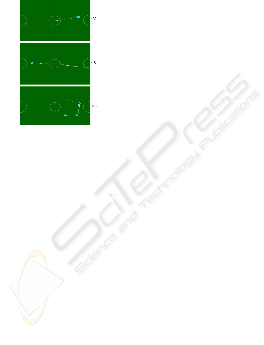
Figure 3: (A) – SetPoint command to x = 0, y = 0. (B) –
setVelocity with v = 0.3mps and desired velocity angle = 0.
(C) – Sequence of setVelocity commands with v = 0.3mps
and velocity angle = 1.3rad.
accurately goes to the defined setPoint, but possess-
ing a yy axis precision error of 1 to 2 centimeters
maximum. This precision error exists because of
two main causes. The first is the backward force
exerted by the energy cable that feeds the robot in test
environment
1
. The second is because of the defined
tuned parameter for the influence of the robot’s error
over the yy coordinate – K
y
. Tuning for near-zero
error is possible but leads to a very hard control
scheme in the presence of a physical disturbance,
making the controller produce high overshoot for
compensation. Since our robot is to walk on a field
where collisions with other robots may be present, the
revealed accuracy perfectly suits for our needs. For
collision-free applications, where minimum physical
errors exist and depending on the world’s space, we
can make the control harder, raising K
y
.
– setVelocity (velocity vector) with v = 0.3mps and
desired velocity angle = 0
For this test, the robot was subjected to extreme noise
conditions.
Referring to Fig. 3(B), the robot is subjected to
two disturbances done by blocking its left wheel,
evident by the multiple white dots in the same place.
Also, we blocked the color code of the robot used to
1
During tests, we prefer to have the robot constantly fed
with energy instead of placing the batteries that discharge
with time.
be identified by the vision module for a while, so that
no vision data was being received by the controller
for it to estimate the actual pose. Controller’s robust-
ness is proved.
– Sequence of setVelocity commands with v = 0.3mps
and velocity angle = 1.3rad
In this final test (Fig. 3(C)), we sent a sequence of
setVelocity commands to evaluate the control mod-
ule’s response in the presence of new velocity in-
structions. This test approaches from our real appli-
cation target, the soccer game, where a high move-
ment dynamic is required for the robot. Referring to
Fig. 3(C), a velocity vector with zero desired angle is
first sent, followed by two setVelocitie’s with the same
module and 1.3 rad for the desired velocity angle. Fi-
nally, the robot is halted with a halt instruction. As we
can conclude, the robot accurately executes the per-
formed commands, evidencing the software module’s
robustness.
7 CONCLUSIONS
A controller for pose error elimination of a soccer-
player robot was projected and its practical results
have been shown. For the theoretical basis of the con-
troller, particular interest was given to create a gen-
eral scheme independent of the mathematical extrac-
tion of the test structure. On-the-field tests reveal that
the projected approach is not only valid, but also ro-
bust. Despite the fact that the Real Time System has
not already been implemented, the idea of placing it in
the system is planned and will be present in the final
version of this project.
REFERENCES
A. Gholipour, M. J. Y. (2000). Dynamic tracking control
of nonholonomic mobile robot with model reference
adaptation for uncertain parameters. University of
Tehran.
T. Larsen, M. B. (2000). Location estimation for an
autonomously guided vehicle using an augmented
kalman filter to autocalibrate the odometry. Techni-
cal University of Denmark.
Y. Kanayama, Y. Kimura, F. M. T. N. (1990). A stable track-
ing control method for an autonomous mobile robot.
IEEE.
ICINCO 2008 - International Conference on Informatics in Control, Automation and Robotics
228
