DESIGN AND IMPLEMENTATION OF A LOW-COST ATTITUDE
AND HEADING NONLINEAR ESTIMATOR
Philippe Martin and Erwan Sala
¨
un
Centre Automatique et Syst
`
emes,
´
Ecole des Mines de Paris, 60 boulevard Saint-Michel, 75272 Paris Cedex 06, France
Keywords:
Observers, sensor fusion, nonlinear filters, strapdown systems, invariance, inertial navigation, extended
Kalman filters.
Abstract:
In this paper we propose a nonlinear observer (i.e. a “filter”) for estimating the orientation of a flying rigid
body, using measurements from low-cost inertial and magnetic sensors. It has by design a nice geometrical
structure appealing from an engineering viewpoint; it is easy to tune, computationally very economic, and with
guaranteed (at least local) convergence around every trajectory. Moreover it behaves sensibly in the presence
of acceleration and magnetic disturbances. We illustrate its good performance on experimental comparisons
with a commercial system, and demonstrate its simplicity by implementing it on a 8-bit microcontroller.
1 INTRODUCTION
Aircraft, especially Unmanned Aerial Vehicles
(UAV), commonly need to know their orientation to
be operated, whether manually or with computer as-
sistance. When cost or weight is an issue, using very
accurate inertial sensors for “true” (i.e. based on the
Schuler effect due to a non-flat rotating Earth) iner-
tial navigation is excluded. Instead, low-cost sys-
tems –often called Attitude Heading Reference Sys-
tems (AHRS)– rely on light and cheap “strapdown”
gyroscopes, accelerometers and magnetometers. The
various measurements are “merged” according to the
motion equations of the aircraft assuming a flat non-
rotating Earth, usually with some kind of Extended
Kalman Filter (EKF). For more details about avionics,
various inertial navigation systems and sensor fusion,
see for instance (Collinson, 2003; Kayton and Fried,
1997; Grewal et al., 2007) and the references therein.
While the EKF is a general method capable of
good performance when properly tuned, it suffers sev-
eral drawbacks: it is not easy to choose the numerous
parameters; it is computationally expensive, which is
a problem in low-cost embedded systems; it is usually
difficult to prove the convergence, even at first-order,
and the designer has to rely on extensive simulations.
An alternative route is to use an ad hoc nonlinear
observer as proposed in (Thienel and Sanner, 2003;
Mahony et al., 2005; Hamel and Mahony, 2006; Mar-
tin and Sala
¨
un, 2007; Mahony et al., 2008). In the
absence of a general method the main difficulty is of
course to find such an observer. In this paper we use
the rich geometric structure of the attitude-heading
problem to derive an observer by the method devel-
oped in (Bonnabel et al., 2007), building up on the
preliminary work (Martin and Sala
¨
un, 2007). It has
by design a nice geometrical structure appealing from
an engineering viewpoint; it is easy to tune, computa-
tionally very economic, and with guaranteed (at least
local) convergence around every trajectory. Moreover
it behaves sensibly in the presence of acceleration and
magnetic disturbances. We illustrate its good perfor-
mance on experimental comparisons with the com-
mercial Microbotics MIDG II system, and demon-
strate its simplicity by implementing it on a 8-bit At-
mel AVR microcontroller.
2 THE PHYSICAL SYSTEM
2.1 Motion Equations
The motion of a flying rigid body (assuming the Earth
is flat and defines an inertial frame) is described by
˙q =
1
2
q ∗ ω
˙
V = A + q ∗ a ∗ q
−1
,
where:
• q is the quaternion representing the orientation of
the body with respect to the Earth-fixed frame
• ω is the instantaneous angular velocity vector
53
Martin P. and Salaün E. (2008).
DESIGN AND IMPLEMENTATION OF A LOW-COST ATTITUDE AND HEADING NONLINEAR ESTIMATOR.
In Proceedings of the Fifth International Conference on Informatics in Control, Automation and Robotics - SPSMC, pages 53-61
DOI: 10.5220/0001502100530061
Copyright
c
 SciTePress

• V is the velocity vector of the center of mass with
respect to the Earth-fixed frame
• A = ge
3
is the (constant) gravity vector in North-
East-Down coordinates (the unit vectors e
1
,e
2
,e
3
point respectively North, East, Down)
• a is the specific acceleration vector, in this case
the aerodynamic forces divided by the body mass.
The first equation describes the kinematics of the
body, the second is Newton’s force law. It is custom-
ary to use quaternions instead of Euler angles since
they provide a global parametrization of the body
orientation, and are well-suited for calculations and
computer simulations. For more details see (Stevens
and Lewis, 2003) or any other good textbook on air-
craft modeling, and section 7 for useful formulas used
in this paper.
2.2 Measurements
We use three triaxial sensors providing nine scalar
measurements: 3 gyros measure ω
m
= ω + ω
b
, where
ω
b
is a constant vector bias; 3 magnetometers mea-
sure y
B
= b
s
q
−1
∗ B ∗ q, where B = B
1
e
1
+ B
3
e
3
is the
Earth magnetic field in NED coordinates and b
s
> 0
is a constant scaling factor; 3 accelerometers measure
a
m
= a
s
a, where a
s
> 0 is a constant scaling factor.
As customary in low-cost unaided attitude heading
systems we assume the linear acceleration
˙
V small,
hence approximate the accelerometers measurements
by y
A
:= a
s
q
−1
∗ A ∗ q (the sign is reversed for conve-
nience). All the nine measurements are of course also
corrupted by noise.
There is some freedom in modeling the sensors
imperfections. A simple first-order observability
analysis reveals that up to six unknown constants can
be estimated: besides the gyro bias ω
b
, it is possible
to estimate two imperfections on y
B
and one on a
m
, or
one on y
B
and two on a
m
. Nevertheless it is impossible
to model three imperfections on a
m
: in particular if
we write a
m
= a + a
b
, with a
b
a constant vector bias,
only two components of a
b
are observable; moreover,
only one imperfection on a
m
can be estimated without
relying on the possibly disturbed magnetic measure-
ments. On the other hand it is also impossible to es-
timate the three components of the magnetic field B,
but only the North and Down components.
In an AHRS it is usually desirable to use the mag-
netic measurements to estimate only the heading, so
that a magnetic disturbance does not affect the es-
timated attitude. We will see this can be achieved
by considering y
C
:= y
A
× y
B
= c
s
q
−1
∗C ∗ q, where
c
s
:= a
s
b
s
> 0 and C := A × B, rather than the direct
measurement y
B
. Notice that hy
A
,y
C
i = hA,Ci = 0, so
that we are left with 8 independent measurements; as
a consequence only five unknown constants can now
be estimated. This is not a drawback and is even ben-
eficial since the observer will then not depend on the
latitude-varying B
3
.
2.3 The Model
To design our observer we thus consider the system
˙q =
1
2
q ∗ (ω
m
− ω
b
) (1)
˙
ω
b
= 0 (2)
˙a
s
= 0 (3)
˙c
s
= 0 (4)
with the output

y
A
y
C

=

a
s
q
−1
∗ A ∗ q
c
s
q
−1
∗C ∗ q

. (5)
This system is observable since all the state vari-
ables can be recovered from the known quantities
ω
m
,y
A
,y
C
and their derivatives: from (5), a
s
=
1
g
k
y
A
k
and c
s
=
1
B
1
g
k
y
C
k
; hence we know the action of q on
the two independent vectors A and C, which com-
pletely defines q in function of y
A
,y
C
,a
s
,c
s
. Finally
(1) yields ω
b
= ω
m
− 2q
−1
˙q.
3 THE NONLINEAR OBSERVER
3.1 Invariance of the System Equations
There is no general method for designing a nonlinear
observer for a given system. When the system has a
rich geometric structure the recent paper (Bonnabel
et al., 2007) provides a constructive method to this
problem. In short, when a system of state dimen-
sion n is invariant by a transformation group of di-
mension r ≤ n, the method yields the general invariant
preobserver. More importantly the error between the
estimated and actual states is described in suitable in-
variant coordinates by a system of dimension 2n − r;
in particular the error system has dimension n when
the group has dimension n. This result, which is rem-
iniscent of the linear case, greatly simplifies the con-
vergence analysis.
In our case the transformation generated by con-
stant rotations and translations in the body-fixed
frame and output scaling
ICINCO 2008 - International Conference on Informatics in Control, Automation and Robotics
54

ϕ
(q
0
,ω
0
,a
0
,c
0
)



q
ω
b
a
s
c
s



=




q ∗ q
0
q
−1
0
∗ ω
b
∗ q
0
+ ω
0
a
0
a
s
c
0
c
s




ψ
(q
0
,ω
0
,a
0
,c
0
)
(ω
m
) = q
−1
0
∗ ω
m
∗ q
0
+ ω
0
ρ
(q
0
,ω
0
,a
0
,c
0
)

y
A
y
C

=

a
0
q
−1
0
∗ y
A
∗ q
0
c
0
q
−1
0
∗ y
C
∗ q
0

,
where q
0
is a unit quaternion, ω
0
a vector in R
3
and
a
0
,c
0
> 0, is easily seen to be a transformation group
with the same dimension as the system (1)–(4).
The system (1)–(4) is indeed invariant by the
transformation group since
˙
z
}|{
q ∗ q
0
= ˙q ∗ q
0
=
1
2
(q ∗ q
0
) ∗

(q
−1
0
∗ ω
m
∗ q
0
+ ω
0
)
− (q
−1
0
∗ ω
b
∗ q
0
+ ω
0
)

˙
z }| {
q
−1
0
∗ ω
b
∗ q
0
+ ω
0
= q
−1
0
∗
˙
ω
b
∗ q
0
= 0
˙
z}|{
a
0
a
s
= a
0
˙a
s
= 0
˙
z}|{
c
0
c
s
= c
0
˙c
s
= 0.
Notice also that from a physical and engineering
viewpoint, it is perfectly sensible for an observer us-
ing measurements expressed in the body-fixed frame
not to be affected by the actual choice of coordinates,
i.e. by a constant rotation in the body-fixed frame.
Similarly, a translation of the gyro bias by a vector
constant in the body-fixed frame and output scalings
should not affect the observer. This is precisely what
the method of (Bonnabel et al., 2007) achieves.
3.2 The General Invariant Observer
Following the theory developed in (Bonnabel et al.,
2007), see also (Martin and Sala
¨
un, 2007) for details,
the general invariant observer writes
˙
ˆq =
1
2
ˆq ∗ (ω
m
−
ˆ
ω
b
) + (LE) ∗ ˆq (6)
˙
ˆ
ω
b
= ˆq
−1
∗ (ME) ∗ ˆq (7)
˙
ˆa
s
= ˆa
s
NE (8)
˙
ˆc
s
= ˆc
s
OE. (9)
Here the invariant output error E is the 5 × 1 vector
E :=

hE
A
,e
1
i,hE
A
,e
2
i,hE
A
,e
3
i,hE
C
,e
1
i,hE
C
,e
2
i

T
made up of the projections of the vectors
E
A
:= A −
1
ˆa
s
ˆq ∗ y
A
∗ ˆq
−1
E
C
:= C −
1
ˆc
s
ˆq ∗ y
C
∗ ˆq
−1
.
Only 5 of the 6 possible projections are independent
since hA,Ci = 0 and hy
A
,y
C
i = 0 imply
hE
A
,E
C
i = hA,E
C
i + hE
A
,Ci;
L,M are 3 × 5 matrices and N,O are 1 × 5 matrices
with entries possibly depending on the components
of E and of the complete invariant I defined by
I := ˆq ∗ (ω
m
−
ˆ
ω
b
) ∗ ˆq
−1
.
It is easy to check this observer is invariant. No-
tice also the two built-in desirable geometric features:
k
ˆq(t)
k
=
k
ˆq(0)
k
= 1 since LE is a vector of R
3
(see
section 7); ˆa
s
(t), ˆc
s
(t) > 0 provided ˆa
s
(0), ˆc
s
(0) > 0.
3.3 The Invariant Error System
Following (Bonnabel et al., 2007), an invariant state
error is given by



η
β
α
γ



=




ˆq ∗ q
−1
q ∗ (
ˆ
ω
b
− ω
b
) ∗ q
−1
a
s
ˆa
s
c
s
ˆc
s




.
Therefore,
˙
η =
˙
ˆq ∗ q
−1
− ˆq ∗ (q
−1
∗ ˙q ∗ q
−1
) = (LE) ∗ η −
1
2
η ∗ β
˙
β = q ∗ (
˙
ˆ
ω
b
−
˙
ω
b
) ∗ q
−1
+ ˙q ∗ (
ˆ
ω
b
− ω
b
) ∗ q
−1
− q ∗ (
ˆ
ω
b
− ω
b
) ∗ q
−1
∗ ˙q ∗ q
−1
= (η
−1
∗ I ∗ η) × β + η
−1
∗ (ME) ∗ η
˙
α = −
a
s
˙
ˆa
s
ˆa
2
s
= −αNE
˙
γ = −
c
s
˙
ˆc
s
ˆc
2
s
= −γOE.
Since E is obtained from
E
A
= A −
a
s
ˆa
s
ˆq ∗ (q
−1
∗ A ∗ q) ∗ ˆq
−1
= A − αη ∗ A ∗ η
−1
E
C
= C − γη ∗C ∗ η
−1
we find as expected that the error system
˙
η = (LE) ∗ η −
1
2
η ∗ β (10)
˙
β = (η
−1
∗ I ∗ η) × β + η
−1
∗ (ME) ∗ η (11)
˙
α = −αNE (12)
˙
γ = −γOE (13)
depends only on the invariant state error (η, β, α, γ)
and the “free” known invariant I, but not on the tra-
jectory of the observed system (1)–(4). This property
greatly simplifies the convergence analysis of the ob-
server.
DESIGN AND IMPLEMENTATION OF A LOW-COST ATTITUDE AND HEADING NONLINEAR ESTIMATOR
55

The linearized error system around the no-error
equilibrium point (η,β,α,γ) = (1,0,1,1) then reads
δ
˙
η = LδE −
1
2
δβ (14)
δ
˙
β = I × δβ + MδE (15)
δ
˙
α = −NδE (16)
δ
˙
γ = −OδE, (17)
where δE is the 5 × 1 vector

hδE
A
,e
1
i,hδE
A
,e
2
i,hδE
A
,e
3
i,hδE
C
,e
1
i,hδE
C
,e
2
i

T
= g

−2δη
2
,2δη
1
,−δα,2B
1
δη
3
,−B
1
δγ

T
made up from the projections of the vectors
δE
A
= A ∗ δη − δη ∗ A − δαA = 2A × δη − δαA
δE
C
= 2C ×δη − δγC.
4 DESIGN OF L,M,N, O
Up to now, we have only investigated the structure of
the observer. We now must choose the gain matri-
ces L,M,N,O to meet the following requirements:
• the error must converge to zero, at least locally
• the local error behavior should be easily tunable,
if possible with a clear physical interpretation
• the magnetic measurements should not affect the
attitude estimate, but only the heading
• the behavior in the face of acceleration and/or
magnetic disturbances should be sensible and un-
derstandable.
4.1 Local Design
It turns out that the previous requirements can easily
be met locally around every trajectory by taking
L :=
1
2g


0 −l
1
0 0 0
l
2
0 0 0 0
0 0 0 −
1
B
1
l
3
0


M :=
1
2g


0 m
1
0 0 0
−m
2
0 0 0 0
0 0 0
1
B
1
m
3
0


N :=
1
g

0 0 −n 0 0

O :=
1
B
1
g

0 0 0 0 −o

for all constant l
1
,l
2
,l
3
,m
1
,m
2
,m
3
,n,o > 0. This will
follow from the very simple form of the linearized er-
ror system (14)–(17). We insist that it is not usually
obvious to come up with a similar convergence result
for an EKF.
Indeed, (14)–(17) now reads
δ
˙
η = D
l
δη −
1
2
δβ (18)
δ
˙
β = D
m
δη + I × δβ (19)
δ
˙
α = −nδα (20)
δ
˙
γ = −oδγ (21)
where
D
l
=


−l
1
0 0
0 −l
2
0
0 0 −l
3


D
m
=


m
1
0 0
0 m
2
0
0 0 m
3


.
When I = 0 (i.e. the system is at rest) the system
completely decouples into:
• the longitudinal subsystem

δ
˙
η
2
δ
˙
β
1

=

−l
1
−
1
2
0 m
1

δη
2
δβ
1

• the lateral subsystem

δ
˙
η
1
δ
˙
β
2

=

−l
2
−
1
2
0 m
2

δη
1
δβ
2

• the heading subsystem

δ
˙
η
3
δ
˙
β
3

=

−l
3
−
1
2
0 m
3

δη
3
δβ
3

• the scaling subsystem
δ
˙
α = −nδα
δ
˙
γ = −oδγ.
When I 6= 0 the longitudinal, lateral and heading sub-
systems are slightly coupled by the biases errors δβ.
We now prove (δη,δβ,δα,δγ) → (0,0,0,0) what-
ever (l
1
,l
2
,l
3
,m
1
,m
2
,m
3
,n,o) > 0. The scaling sub-
system obviously converges. For the other variables
we consider the Lyapunov function
V =
l
1
2
δη
2
1
+
l
2
2
δη
2
2
+
l
3
2
δη
2
3
+
1
4
kδβk
2
.
Differentiating V and using hδβ, I × δβi = 0, we get
˙
V = − (l
1
m
1
δη
2
1
+ l
2
m
2
δη
2
2
+ l
3
m
3
δη
2
3
) ≤ 0.
Since V is bounded from below, this implies that
V (δη(t),δβ(t)) converges as t → ∞. Since
lim
t→∞
Z
t
0
˙
V (δη(τ),δβ(τ))dτ = lim
t→∞
V (δη(t),δβ(t))
−V (δη(0),δβ(0)),
ICINCO 2008 - International Conference on Informatics in Control, Automation and Robotics
56

we conclude lim
t→∞
R
t
0
˙
V (δη(τ),δβ(τ))dτ exists and
is finite. On the other hand,
˙
V ≤ 0 also implies
0 ≤ V (δη(t),δβ(t)) ≤ V (δη(0),δβ(0)).
Therefore δη(t) and δβ(t) are bounded. Equation
(18) implies that δ
˙
η(t) is bounded too, and finally that
¨
V is bounded. Hence
˙
V is uniformly continuous and
by Barbalat’s lemma
˙
V → 0 ⇒ δη → 0.
Integrating (18), we get
Z
t
0
δ
˙
η(τ)dτ = δη(t) − δη(0)
=
Z
t
0
(D
l
δη(τ) −
1
2
δβ(τ))dτ.
Since δη(t) → 0, it follows
lim
t→∞
Z
t
0
(D
l
δη(τ) −
1
2
δβ(τ))dτ = −δη(0).
We assume I is bounded, which is physically sensible.
Since δη(t) and δβ(t) are bounded, D
l
δ
˙
η(t) −
1
2
δ
˙
β(t)
is bounded too. Hence D
l
δη(t) −
1
2
δβ(t) is uniformly
continuous. Applying Barbalat’s lemma once again
yelds
lim
t→∞
(D
l
δη(t) −
1
2
δβ(t)) = 0.
Since δη → 0, we conclude δβ → 0, which ends the
proof.
4.2 Global Design
We now look for correction terms ensuring global
convergence whereas preserving the previous nice
first-order properties. It is useful to define the fol-
lowing vectors and error output:
D = C × A
y
D
= y
C
× y
A
E
D
= D −
1
ˆa
s
ˆc
s
ˆq ∗ y
D
∗ ˆq
−1
.
If we define the matrix L by
LE :=
l
a
g
2
A × E
A
+
l
c
(B
1
g)
2
C × E
C
+
l
d
(B
1
g
2
)
2
D × E
D
it is easy to see that the zero-order part of L is the
same as the constant L of section 4.1 with
l
1
= l
a
+ l
c
l
2
= l
a
+ l
d
l
3
= l
c
+ l
d
.
To find a candidate Lyapunov function we also select
the matrices (M,N,O) by
ME := σLE
NE := n

l
a
g
2
E
T
A
(E
A
− A) +
l
d
(B
1
g
2
)
2
E
T
D
(E
D
− D)

OE := o

l
c
(B
1
g)
2
E
T
C
(E
C
−C) +
l
d
(B
1
g
2
)
2
E
T
D
(E
D
− D)

with (l
a
,l
c
,l
d
,σ,n,o) > 0. The positive function V :=
1
σ
k
β
k
2
+
l
a
g
2
k
E
A
k
2
+
l
c
(B
1
g)
2
k
E
C
k
2
+
l
d
(B
1
g
2
)
2
k
E
D
k
2
satisfies
˙
V ≤ 0. The convergence proof follows the
main lines of (Hamel and Mahony, 2006), with added
technicalities.
With these choices the first-order behavior is the
same as in section 4.1. The difference is the existence
of the proportional factor σ between the l
0
i
s, m
0
i
s co-
efficients. We now have only 4 independent gains for
the lateral, longitudinal and heading subsystems in-
stead of 6. We choose to fix first the natural frequen-
cies of the lateral (ω
l
), longitudinal (ω
L
) and heading
(ω
h
) subsystems. There is only 1 parameter left to fix
the free damping ratios.
5 EFFECTS OF DISTURBANCES
Two main disturbances may affect the model.
When
˙
V 6= 0, the accelerometers measure in fact
a
s
q
−1
∗ A
∗
∗ q where A
∗
:= −
˙
V + A. Magnetic distur-
bances will also change B into some B
∗
. For simplic-
ity we consider that A
∗
, B
∗
are constant. The mea-
sured outputs now become

y
A
∗
y
C
∗

=

a
s
q
−1
∗ A
∗
∗ q
c
s
q
−1
∗C
∗
∗ q

.
The error system is unchanged but E is now the 5 × 1
vector
E :=

hE
A
,e
1
i,hE
A
,e
2
i,hE
A
,e
3
i,hE
C
,e
1
i,hE
C
,e
2
i

T
made up of the projections of the vectors
E
A
:= A −
1
ˆa
s
ˆq ∗ y
A
∗
∗ ˆq
−1
E
C
:= C −
1
ˆc
s
ˆq ∗ y
C
∗
∗ ˆq
−1
.
Let us define the points (η,β,α,γ) as following
β = 0
η ∗ A
∗
∗ η
−1
= (0 0
k
A
∗
k
)
η ∗C
∗
∗ η
−1
= (0
k
C
∗
k
0)
α =
k
A
∗
k
k
A
k
and γ =
k
C
∗
k
k
C
k
DESIGN AND IMPLEMENTATION OF A LOW-COST ATTITUDE AND HEADING NONLINEAR ESTIMATOR
57

Doing the frame rotation defined by η we can define
the new variables
˜
η = η ∗ η
−1
˜
β = η ∗ β ∗ η
−1
˜
α = αα
˜
γ = γγ.
The error system with these new variables writes
˙
˜
η = −
1
2
˜
η ∗
˜
β + (
˜
L
˜
E) ∗
˜
η
˙
˜
β = (
˜
η
−1
∗
˜
I ∗
˜
η) ×
˜
β +
˜
η
−1
∗ (
˜
M
˜
E) ∗
˜
η
˙
˜
α = −
˜
α
˜
N
˜
E
˙
˜
γ = −
˜
γ
˜
O
˜
E
where the new output error
˜
E is made up of the pro-
jections of the vectors
˜
E
A
= A −
˜
α
˜
η ∗ A ∗
˜
η
−1
˜
E
C
= C −
˜
α
˜
η ∗C ∗
˜
η
−1
.
So (
˜
η,
˜
β,
˜
α,
˜
γ) verify the same error system as
(η,β,α,γ). In the new frame (A
∗
,C
∗
) play the same
role as (A,C). All the properties of the observer are
therefore preserved.
An important case is when only the magnetic field
is perturbed, where we consider A and C
∗
= (C
∗
1
C
∗
2
0)
(instead of C = (0 gB
1
0)). Expliciting the new equi-
librium point (η,β,α,γ) of the error system it can be
seen that
φ = θ = 0 and ψ = arctan
C
∗
1
C
∗
2
β = α = 0 and γ =
k
C
∗
k
k
C
k
,
where (φ, θ, ψ) are the Euler angles corresponding to
η. In particular only the yaw angle ψ and γ are af-
fected by the magnetic disturbance.
6 EXPERIMENTAL VALIDATION
We now compare the behavior of our observer with
the commercial Microbotics MIDG II system used in
Vertical Gyro mode. The following results have been
obtained with the observer
˙
ˆq =
1
2
ˆq ∗ (ω
m
−
ˆ
ω
b
) + (LE) ∗ ˆq + k(1 −
k
ˆq
k
2
) ˆq
˙
ˆ
ω
b
= ˆq
−1
∗ (ME) ∗ ˆq
˙
ˆa
s
= ˆa
s
NE
˙
ˆc
s
= ˆc
s
OE
and the choice of matrices defined by the parameters
below. The added term k(1 −
k
ˆq
k
2
) ˆq is a well-known
numerical trick to keep
k
ˆq
k
= 1. Notice this term is
also invariant.
We feed the observer with the raw measurements
from the MIDG II gyros, acceleros and magnetic
sensors. The observer is implemented in Matlab
Simulink and its values are compared to the MIDG II
results (computed according to the user manual by
some Kalman filter). In order to have similar behav-
iors, we have chosen
l
a
= 6e − 2 l
c
= 1e − 1 l
d
= 6e − 2
m
a
= 3.2e − 3 m
c
= 5.3e − 3 m
d
= 3.2e − 3
n = 0.25 o = 0.5.
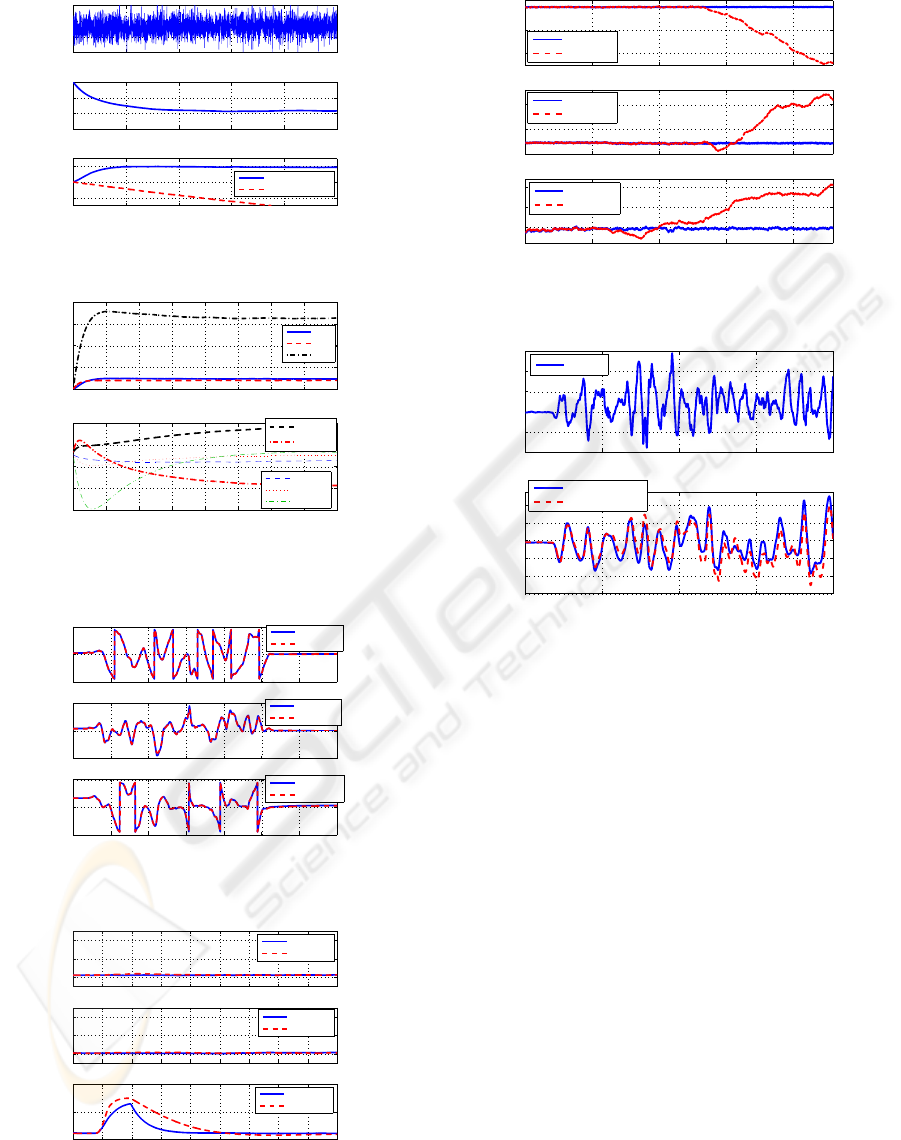
6.1 Comparison with a Commercial
Device (Figure 1)
We first want to put in evidence the different proper-
ties of our observer we mentioned before. Therefore
we did a long experience which can be divided into 3
parts:
• for t < 240s the system is left at rest until the
biases reach constant values. Fig.1(a) highlights
the importance of the correction term in the angle
estimation: without correction the estimated roll
angle diverges with a slope of −0.18
◦
/s (bottom
plot), which is indeed the final value of the esti-
mated bias (middle plot) (Fig.1(a) and 1(b)).
• for 240s < t < 293s we move the system in all di-
rections. The observer and the MDG II give very
similar results (Fig.1(c)).
• at t = 385s the system is motionless and a magnet
is put close to the sensors for 10s. As expected
only the estimated yaw angle is affected by the
magnetic disturbance (Fig.1(d)); the MIDG II ex-
hibits a similar behavior.
6.2 Influence of the Observer
Correction Terms (Figure 2)
We have chosen the correction terms so as the mag-
netic measurements correct essentially the yaw angle
and its corresponding bias, whereas the accelerom-
eters measurements act on the other variables. We
highlight this property on the following experiment
(Fig.2). Once the biases have reached constant val-
ues, the system is left at rest during 35 minutes:
• for t < 600s the results are very similar for the
observer and the MIDG II.
• at t = 600s the “magnetic correction terms” are
switched off, i.e. the gains l
c
,l
d
,m
c
,m
d
and o are
ICINCO 2008 - International Conference on Informatics in Control, Automation and Robotics
58

0 20 40 60 80 100
−1
−0.5
0
0.5
Measured roll angular rate
(°/s)
0 20 40 60 80 100
−0.2
−0.1
0
Estimated roll angular rate bias
(°/s)
0 20 40 60 80 100
−10
0
10
Estimated roll angle
time(s)
(°)
With correction
Without correction
(a) Motionless estimated roll angle.
0 20 40 60 80 100 120 140 160
0
20
40
60
80
Estimated Euler angles
(°)
Roll
Pitch
Yaw
0 20 40 60 80 100 120 140 160
−1.4
−0.85
−0.3
0.25
0.8
time (s)
(°/s)
Estimated biases and scalings
0 20 40 60 80 100 120 140 160
0.7
0.775
0.85
0.925
1
Roll bias
Pitch bias
Yaw bias
Scaling a
s
Scaling c
s
(b) Motionless estimated gyros biases and Eu-
ler angles.
240 250 260 270 280 290 300 310
−200
0
200
Estimated Euler angles
(°)
φ MIDGII
estimated φ
240 250 260 270 280 290 300 310
−100
0
100
(°)
θ MIDGII
estimated θ
240 250 260 270 280 290 300 310
−200
0
200
time(s)
(°)
ψ MIDGII
estimated ψ
(c) Dynamic estimated Euler angles.
380 390 400 410 420 430 440 450 460 470
0
10
20
Estimated Euler angles with magnetic disturbance
(°)
380 390 400 410 420 430 440 450 460 470
0
10
20
(°)
380 390 400 410 420 430 440 450 460 470
0
50
100
time(s)
(°)
φ MIDGII
estimated φ
θ MIDGII
estimated θ
ψ MIDGII
estimated ψ
(d) Estimated Euler angles with magnetic dis-
turbances.
Figure 1: Experimental validation using Matlab.
0 500 1000 1500 2000
−20
−10
0
Estimated Euler angles
(°)
φ MIDGII
estimated φ
0 500 1000 1500 2000
−5
0
5
(°)
θ MIDGII
estimated θ
0 500 1000 1500 2000
140
145
150
time(s)
(°)
ψ MIDGII
estimated ψ
Figure 2: Influence of correction terms.
180 185 190 195 200
0
500
1000
1500
2000
2500
Estimations of the roll angle with acceleration
milli−g
180 185 190 195 200
−60
−40
−20
0
20
40
(°)
time(s)
norm(y
A
)
θ MIDGII with GPS
estimated θ
Figure 3: Estimated roll angle at
˙
V 6= 0.
set to 0. The yaw angle estimated by the ob-
server diverges because the corresponding bias is
not perfectly estimated. Indeed, these variables
are not observable without the magnetic measure-
ments. The other variables are not affected.
• at t = 1300s the “accelerometers correction
terms” are also switched off, i.e. l
a
,m
a
and n are
set to 0. All the estimated angles now diverge.
6.3 Acceleration Disturbance:
˙
V 6= 0
(Figure 3)
The hypothesis
˙
V = 0 may be wrong. In this case the
observer does not converge any more to the right val-
ues. Indeed we illustrate this point on the figure 3 by
comparing the roll angle estimated by our observer
and the roll angle estimated by the MIDG II in INS
mode (in this mode the attitude and heading estima-
tions are aided by a GPS engine, hence are close to
the “true” values).
DESIGN AND IMPLEMENTATION OF A LOW-COST ATTITUDE AND HEADING NONLINEAR ESTIMATOR
59

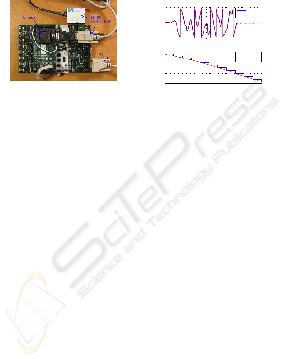
Figure 4: Experimental protocol.
7 IMPLEMENTATION ON A 8-BIT
MICROCONTROLLER
In the preceding section we validated the Matlab
Simulink implementation of our observer. To demon-
strate its computational simplicity we have also im-
plemented it on a 8-bit microcontroller (Atmel AT-
mega128 running at 11.0592MHz on development kit
STK500/501). The computations are done in C with
the standard floating point emulation. The microcon-
troller is fed with the MIDG II raw data at a 50Hz rate.
We have used a simple Euler explicit approximation
for the integration scheme.
The experimental protocol was the following:
1. move the sensors in all directions and save the
MIDG II raw measurements and estimations at
50Hz.
2. use of xPCTarget to feed the ATmega with these
data at 50Hz via a serial port and send at the same
time the estimated variables. given by the micro-
controller via a serial port to a computer
3. save these estimations.
4. compare offline the estimations given by the mi-
crocontroller and those given by the observer writ-
ten in the Matlab embedded function.
This protocol can be illustrated by the figure 4 where
xPCTarget has been replaced by the MIDG II.
We obtain the results of the figure 5. The two es-
timations are very similar. We see on the bottom plot
the discretization at 50Hz due to the microcontroller.
REFERENCES
Bonnabel, S., Martin, P., and Rouchon, P. (2007). Invari-
ant observers. arxiv.math.OC/0612193. Accepted for
publication in IEEE Trans. Automat. Control.
240 250 260 270 280 290 300 310
−200
−100
0
100
200
Comparison ATmega/Matlab
(°)
253.25 253.3 253.35 253.4
70
75
80
85
90
(°)
time(s)
φ ATmega
φ Matlab
φ ATmega
φ Matlab
Figure 5: Comparison ATmega/Matlab.
Collinson, R. (2003). Introduction to avionics systems.
Kluwer Academic Publishers, second edition.
Grewal, M., Weill, L., and Andrews, A. (2007). Global po-
sitioning systems, inertial navigation, and integration.
Wiley, second edition.
Hamel, T. and Mahony, R. (2006). Attitude estimation
on SO(3) based on direct inertial measurements. In
Proc. of the 2006 IEEE International Conference on
Robotics and Automation, pages 2170–2175.
Kayton, M. and Fried, W., editors (1997). Avionics naviga-
tion systems. Wiley, second edition.
Mahony, R., Hamel, T., and Pfimlin, J.-M. (2008). Non-
linear complementary filters on the special orthogonal
group. IEEE Trans. Automat. Control. To appear.
Mahony, R., Hamel, T., and Pflimlin, J.-M. (2005). Comple-
mentary filter design on the special orthogonal group
SO(3). In Proc. of the 44th IEEE Conf. on Decision
and Control, pages 1477–1484.
Martin, P. and Sala
¨
un, E. (2007). Invariant observers for
attitude and heading estimation from low-cost inertial
and magnetic sensors. In Proc. of the 46th IEEE Conf.
on Decision and Control.
Stevens, B. and Lewis, F. (2003). Aircraft control and sim-
ulation. Wiley, second edition.
Thienel, J. and Sanner, R. (2003). A coupled nonlinear
spacecraft attitude controller and observer with an un-
known constant gyro bias and gyro noise. IEEE Trans.
Automat. Control, 48(11):2011–2015.
APPENDIX: QUATERNIONS
Thanks to their four coordinates, quaternions provide
a global parametrization of the orientation of a rigid
body (whereas a parametrization with three Euler an-
gles necessarily has singularities). Indeed, to any
quaternion q with unit norm is associated a rotation
matrix R
q
∈ SO(3) by
q
−1
∗~p ∗ q = R
q
·~p for all ~p ∈ R
3
.
ICINCO 2008 - International Conference on Informatics in Control, Automation and Robotics
60

A quaternion p can be thought of as a scalar
p
0
∈ R together with a vector ~p ∈ R
3
,
p =

p
0
~p

.
The (non commutative) quaternion product ∗ then
reads
p ∗ q ,

p
0
q
0
−~p ·~q
p
0
~q + q
0
~p +~p ×~q

.
The unit element is e ,

1
~
0

, and
(p ∗ q)
−1
= q
−1
∗ p
−1
.
Any scalar p
0
∈ R can be seen as the quaternion

p
0
~
0

, and any vector ~p ∈ R
3
can be seen as the
quaternion

0
~p

. We systematically use these iden-
tifications in the paper, which greatly simplifies the
notations.
We have the useful formulas
p × q , ~p ×~q =
1
2
(p ∗ q − q ∗ p)
(~p ·~q)~r = −
1
2
(p ∗ q + q ∗ p) ∗ r.
If q depends on time, then ˙q
−1
= −q
−1
∗ ˙q ∗ q
−1
.
Finally, consider the differential equation
˙q = q ∗ u + v ∗ q where u,v are vectors ∈ R
3
. Let q
T
be defined by

q
0
−~q

. Then q∗q
T
=
k
q
k
2
. Therefore,
˙
z}|{
q ∗ q
T
= q ∗ (u + u
T
) ∗ q
T
+
k
q
k
2
(v + v
T
) = 0
since u, v are vectors. Hence the norm of q is con-
stant.
DESIGN AND IMPLEMENTATION OF A LOW-COST ATTITUDE AND HEADING NONLINEAR ESTIMATOR
61