VISUAL TRACKING ON THE GROUND

A Comparative Analysis

Jorge Raul Gomez, Jose J. Guerrero and Elias Herrero-Jaraba

Aragon Institute for Engineering Research, University of Zaragoza, Maria de Luna 1, Zaragoza, Spain

Keywords:

Tracking on the ground, Kalman ﬁlter, Homography.

Abstract:

Tracking is an important ﬁeld in visual surveillance systems. Trackers have been applied traditionally in the

image, but a new concept of tracking has been used gradually, applying the tracking on the ground map of the

surrounding area. The purpose of this article is to compare both alternatives and prove that this new usage

makes possible to obtain a higher performance and a minimization of the projective effects. Moreover, it

provides the concept of multi-camera as a new tool for mobile object tracking in surveillance scenes, because

a common reference system can be deﬁned without increasing complexity. An automatic camera re-calibration

procedure is also proposed, which avoids some practical limitations of the approach.

1 INTRODUCTION

Real-time object tracking is recently becoming more

and more important in the ﬁeld of video analysis and

processing. Applications like trafﬁc control, user-

computer interaction, on-line video processing and

production and video surveillance need reliable and

economically affordable video tracking tools. In the

last years this topic has received an increasing at-

tention by researchers. However, many of the key

problems are still unsolved. The surveillance track-

ing community in particular has studied target track-

ing techniques for a number of years, mainly in the

context of ﬁnding efﬁcient methods to track missiles,

aircrafts etc. and tracking targets of unknown motion.

Their work has been used for a variety of applications.

There have been previous contributions in order

to improve such systems. Tissainayagam and Suter

(Tissainayagam and Suter, 2001) proposed a tracking

method in which a model switching was used. Other

authors, as Isler (Isler et al., 2005), use the technique

of multiple or distributed sensors, assigning sensors

to track targets so as to minimize the expected error in

the resulting estimation for target locations. In most

of the cases, the sensors used for these tasks are inher-

ently limited, and individually incapable of estimating

the target state, and they only can be used for a unique

task. This limitation disappears with the use of cam-

eras. In this way, Lee et al. (Lee et al., 2000) sug-

gested to establish a common coordinate frame and to

capture image signals from several cameras arranged

in a particular environment. This last idea is used in

this paper in order to demonstrate that this solution

contributes a better solution to the tracking problem.

We propose a simple tracker based on the Kalman

Filter. This tracker is used in two different ways (on

the image plane and on the ground plane), making

a comparative between both. Theoretically, the per-

spective effects must disappear in the second one, and

therefore, the tracking must involve better. This paper

shows this event such in laboratory conditions as in

real environments.

This paper is organized as follows: Section 2

brieﬂy details the transformation between the image

and the ground. After that an automatic re-calibration

procedure that avoids some of the practical limitations

of the approach is proposed. Section 3 provides de-

tails of the tracking on the ﬂoor, showing the differ-

ent stages of the proposed tracking system: detection,

tracking, uncertainty transformation, and tuning. In

Section 4 we provide our results in a particular envi-

ronment (our laboratory) under stable conditions. Fi-

nally, some results for a more complex environment

(a football match) are shown also in section 4.

Raul Gomez J., J. Guerrero J. and Herrero-Jaraba E. (2008).

VISUAL TRACKING ON THE GROUND - A Comparative Analysis.

In Proceedings of the Fifth International Conference on Informatics in Control, Automation and Robotics - RA, pages 45-52

DOI: 10.5220/0001487400450052

 SciTePress

2 FROM IMAGE TO THE

GROUND

In order to transform the coordinates from the image

to the planar ground, a plane projection transforma-

tion is used. At the moment no distortion of the cam-

era lens is assumed. A point in the projective plane

is represented by three coordinates, p = (x

)

which represents a ray through the origin in the 3D

space (Mundy and Zisserman, 1992). Only the di-

rection of the ray is relevant, so all points written as

λp = (λx

,λx

)

are equivalent. The classical

Cartesian coordinates of the point (x,y) can be ob-

tained intersecting the ray with a special plane per-

pendicular to x

axis and located at unit distance along

. This is equivalent to scale p as, p = (x,y,1)

. Pro-

jected points in an image and real points in a planar

ground are both represented in this way.

A projective transformation between two projec-

tive planes (1 and 2) can be represented by a linear

transformation p

= T

. If the transformation is

represented in Cartesian coordinates it results non-

linear. Since points and lines are dual in the projec-

tive plane, the transformation for the line coordinates

is also linear, being



−1



the corresponding trans-

formation matrix for lines.

2.1 Computing the Transformation to

Calibrate the Camera

Let it be p

= (x

,1)

the coordinates of a point i

in the camera reference system. Let it be (x

) the

coordinates of the corresponding point in a reference

system of the planar ground obtained from the plane

of the building, and therefore let it be p

= (x

,1)

its homogeneous coordinates.

Figure 1: Diagram depicting the transformation of coordi-

nates from image to the ground.

We obtain the projective transformation T

up to

a non-zero scale factor, for points, p

= T

. For

each couple i of corresponding points, two homo-

geneous equations to compute the projective trans-

formation are considered. They can be written as,

(λ

,λ

)

= T

,1)

. Developing them in

function of the elements of the homography matrix,

we have



1 0 0 0 −x

−x

0 0 0 x

1 −y

−y



t =





where t = (t

)

is a vector

with the elements of the homography matrix T

Using four pairs of corresponding points (no three

of them being collinear), we can construct a 8x9 ma-

trix M, where Mt = 0. Then, the solution t corre-

sponds with the eigenvector associated to the least

eigenvalue (in this case the null eigenvalue) of the

matrix M

M, which can be easily solved by singu-

lar value decomposition (svd) of matrix M. In order

to have a reliable transformation, more than the min-

imum number of point correspondences must be con-

sidered, solving in a similar way (Hartley and Zisser-

man, 2000).

It is known that a previous normalization of data

is suitable to avoid numerical computation problems

(Hartley, 1997). We have transformed the coordinates

of the points (in the image and in the ground) before

the computation of the homography to reference sys-

tems located in the centroid of the points and scaled

in such that the maximum distance of the points to its

centroid is 1. After computation of the homography,

it is inversely transformed by simple matrix compu-

tation to express the homography in the desired refer-

ence systems.

2.2 Automatic Camera Re-calibration

Once we have calibrated the camera using at least 4

pairs of corresponding points in the image and in the

ground, it cannot be moved, which is the main lim-

itation of this proposal. In practice, due for exam-

ple to the ﬂexibility of the camera support, the ori-

entation of the camera changes. A little change of

orientation has a great inﬂuence in the image coor-

dinates of a point, and therefore invalidates previous

calibration. However if the camera is not changed in

position, or position change is small with respect to

the depth of the observed scene, the homography can

be re-calibrated automatically with high robustness

and without 3D computations. As camera position

changes suppose main reconﬁguration of the surveil-

lance system, but orientation changes are usual, the

automatic re-calibration procedure presented below

eliminates the limitation in practice. Besides that, this

re-calibration procedure can also be used for changes

in zoom lens or motions in pan-tilt cameras demanded

by the user.

The re-calibration can be made using features ex-

tracted in the image like points and/or lines. We pro-

pose to do it using lines because they are plentiful in

ICINCO 2008 - International Conference on Informatics in Control, Automation and Robotics

man made environments and have other advantages.

The straight lines have a simple mathematical repre-

sentation, they can be extracted more accurately than

points being also easier to match them and they can

be used in cases where there are partial occlusions.

After extracting the lines, automatic computa-

tion of correspondences and homographies is car-

ried out, as previously presented in (Guerrero and

Sag

es, 2003), which uses robust estimation tech-

niques. Thus, initially the extracted lines are matched

to the weighted nearest neighbor using brightness-

based and geometric-based image parameters.

With the coordinates of at least four pairs of cor-

responding lines we can obtain an homography that

transforms both images. As usually we have many

more than four line correspondences, an estimation

method can be used to process all of them, getting bet-

ter results. The least squares method assumes that all

the measures can be interpreted with the same model,

which makes it to be very sensitive to wrong corre-

spondences. The solution is to use robust estimation

techniques which detect the outliers in the computa-

tion. From the existing robust estimation methods,

we have chosen the least median of squares method

(Rousseeuw and Leroy, 1987).

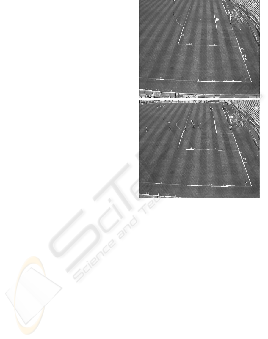
In ﬁgure 2 we can see an example of two images

before and after an unexpected camera motion. The

automatic robust matching of lines that allows to com-

pute the camera re-calibration has been superimposed

to the images. The initial matching has about 20% of

wrong correspondences, but the robust computation

of the homography allows to reject wrong matches

and also to search more matches according to it in a

subsequent step. From the line correspondences the

homography to recalibrate the camera is accurately

obtained.

3 TRACKING ON THE GROUND

3.1 Detection and Tracking

A widely used technique for separating moving ob-

jects from their backgrounds is based on background

subtraction (Herrero et al., 2003). In this approach,

an image I

(x,y) of the background is stored before

the introduction of a foreground object. Then, given

an image I(x,y) from a sequence, feature detection of

moving objects are restricted to areas of I(x, y) where:

|I(x, y) −I

(x,y)| > σ (1)

where σ is a suitable chosen noise threshold.

But this approach exhibits poor results in most real

image sequences due to four main problems:

Figure 2: Two images of a football match before and after

an unexpected camera motion in a real application. The au-

tomatic robust line correspondences has been superimposed

to the images.

• Noise in the image.

• Gray level similarity between background and

moving objects, even if the color is different.

• Continuous or quick illumination changes in the

scene.

• Variation of the static objects in the background.

These problems can be partially solved by an appro-

priate selection of the threshold value. Some authors

(Durucan and Ebrahimi, 2001) (Fabrice Moscheni

and Kunt, 1998) have proposed a region-based motion

segmentation using adaptive thresholding, according

to illumination changes. In addition to this, morpho-

logical ﬁlters have to be used to eliminate noisy pix-

els and to ﬁll the moving regions poorly segmented.

However, in spite of these improvements, the results

that can be found in real situations are far away from

a satisfactory solution.

To detect the moving objects, we present an ap-

VISUAL TRACKING ON THE GROUND - A Comparative Analysis

proach in motion detection, based on difference, in-

troducing two procedures, Neighborhood-Based De-

tection and Overlapping-Based Labelling, in order to

obtain a more robust segmentation in real scenes. The

ﬁrst one uses a local convolution mask, instead of

a punctual one, to compute difference and obtain a

more reliable difference image. The second one uses

an overlapping criterion between two difference im-

age to classify blobs in two different types: static or

dynamic. This last characteristic makes a distinction

between moving objects and shadows or illumination

changes.

After the motion detection, a Kalman tracker

(Kalman, 1960) with a constant velocity model (Bar-

Shalom and Fortmann, 1988) is used for tracking, us-

ing the center of each detected object as measure data.

Internally, the tracker has a state with 4 elements: 2

for the position and 2 for the velocity.

The Kalman ﬁlter is divided in two main parts:

prediction and estimation. Between them, a match-

ing procedure associates the measures obtained in the

motion detection with the prediction of the tracking.

It select the nearest-neighbor if it is close enough in

function of the covariance of the innovation.

3.2 Uncertainty Transformation

The measure in the Kalman tracker is the position

(x,y) of the mobile object. The measure noise has

pixel units, but in order to do the tracking in the

ground, it must be transformed according to the ho-

mography to metric units. To transform the covari-

ance matrix from image to ground, as proposed in

(A. Criminisi and Zisserman, 1997), a transformation

in three steps is required: change to homogeneous co-

ordinates, transformation of coordinates from image

to ground and transformation to inhomogeneous co-

ordinates again.

Given a covariance matrix, which express the un-

certainty location in image coordinates:

2×2





(2)

the correspondent homogeneous one is obtained:



2×2



(3)

The change of homogeneous coordinates from im-

age to the ground is made with the homography ma-

trix T

. Therefore, the covariance matrix is trans-

formed as:

= T

(4)

Once we have the uncertainty in the ground in ho-

mogeneous coordinates, we need to transform to non-

homogeneous coordinates in order to have the mea-

surement. We will use ∇ f as a ﬁrst-order approxi-

mation of the relationship between homogeneous and

inhomogeneous coordinates. If X

= (X ,Y,W )

∇ f = 1/W



W 0 −X

0 W −Y



(5)

Therefore, the covariance matrix of the measure-

ments noise in ground coordinates is

2×2

= ∇ f Λ

∇ f

(6)

This transformation allows to have a noise model

which considers the inﬂuence of the perspective effect

when we made the tracking in the ground.

3.3 Tuning in Practice

The constant velocity model only can be considered

locally valid. In practice, there are velocity changes

that we model in the process noise. If we consider

that the goal have an acceleration which is modelled

as a white noise with zero mean and covariance q

, the

state noise matrix Q

for each coordinate i = x

(Bar-Shalom and Fortmann, 1988):

= q

(7)

where dt is the time interval.

If we consider the tracker in the ground, the tun-

ing has a well known meaning, because

√

repre-

sents directly the acceleration of the mobile. On the

other hand, the classical tracker in the image needs

an empirical tuning in pixel units, that depends of the

perspective effect.

The measure noise matrix R is deﬁned in the im-

age for both trackers and transformed to the ground

using the homography matrix for the tracker on the

ground, as seen in section 3.2.

4 EXPERIMENTS

4.1 Description

The objective of these experiments is to compare

the performance of a tracker on the ground versus a

tracker on the image. Two Kalman trackers will be

compared, using the same constant velocity model,

although each one may have a different, but equiva-

lent, tuning, since coordinates in the image and coor-

dinates in the ground represent different magnitudes.

The three ﬁrst tests performed compare the preci-

sion of the predictions of both trackers in a sequence

ICINCO 2008 - International Conference on Informatics in Control, Automation and Robotics

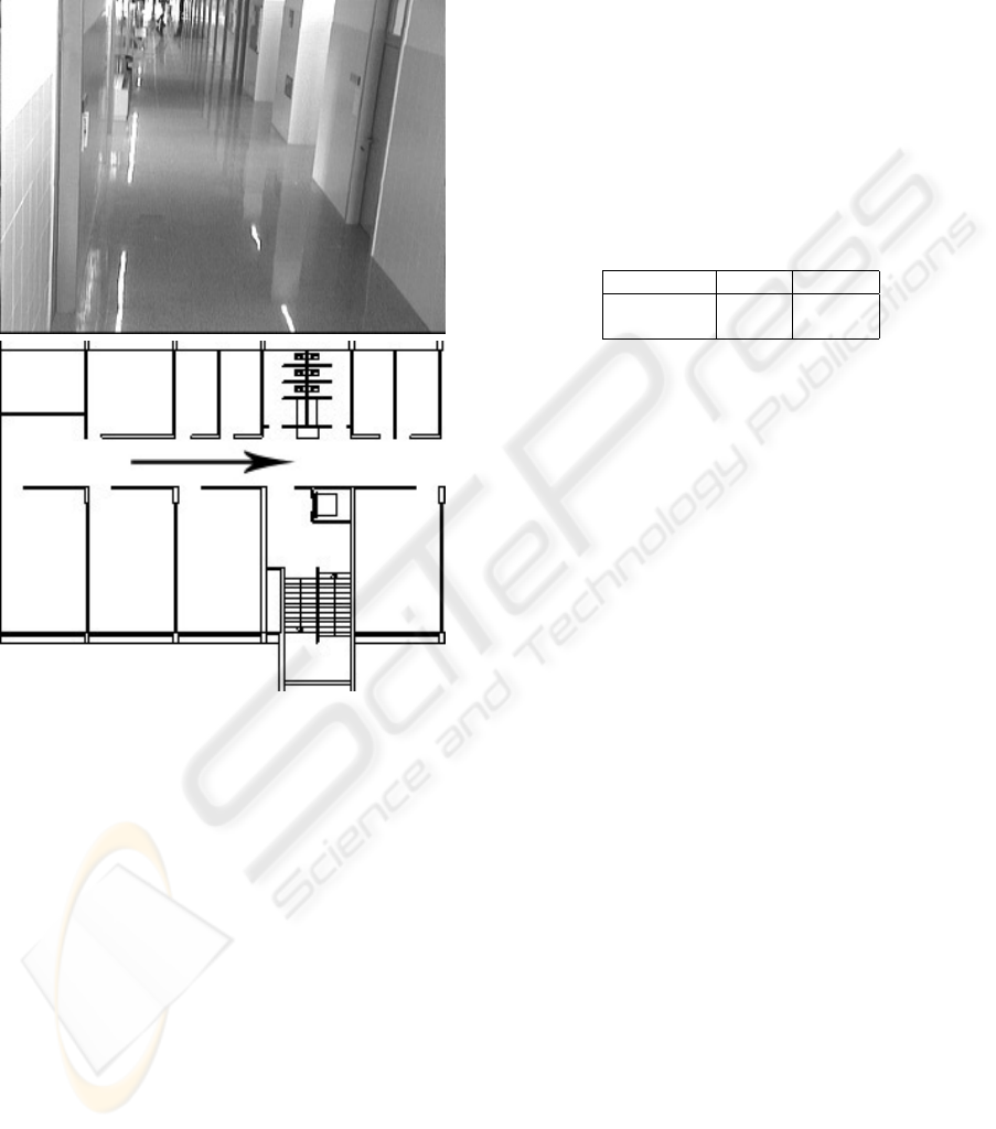
of 550 frames, recorded with a still camera located

in a corridor at 2.5 meters high. The target is a

remote-controlled car moving at nearly constant ve-

locity though a corridor, as it can be seen in ﬁg. 3.

Figure 3: First image of the sequence (up) and building

plane (down) where the tests have been performed. The

remote-controlled car moves along the corridor in the tests,

as the arrow shows.

After obtaining the position of the car in each

frame, a tracker on the image has been applied. At

the same time, the homography previously calculated,

allows us to obtain the corresponding points in the

ground for each point in the image, making possi-

ble to track the same object with another independent

similar tracker on the ground.

To compare the performance of these two track-

ers, the mean difference between the prediction points

and their corresponding measures has been computed.

This difference is only taken into account if the

measure is considered to belong to the object being

tracked. Predictions from these two trackers are go-

ing to be compared at three levels: short, medium and

long-term.

4.2 Comparative Analysis

Test 1: The ﬁrst test compares the precision of short-

term predictions. In the original sequence, the object

is moving away the camera, with occasional lateral

movements. The sequence will be tested also in re-

verse mode, starting from the last frame to the ﬁrst,

making the target go towards the camera. Mean dis-

tances obtained between prediction and measures, de-

noted as d

, are shown in table 1. All distances are

measured in the ground, using Euclidean distance.

Table 1: Mean distances in mm. between predictions and

measures for the image tracker and the ground tracker with

the sequence processed forwards and backwards.

Image Ground

Forwards 54,90 18,89

Backwards 44,02 20,01

In this ﬁrst test, a tracking on the ground has a

great advantage over a tracking on the image, since

the effect of the perspective deformation is avoided.

Distances between predictions and measures are rep-

resented in ﬁgure 4.

As it can be seen in ﬁgure 4, a tracker on the

ground obtains better results if the moving object is

near the camera, because the velocity of the object in

the image is more changeable. However, a tracker on

the image obtains opposite results, since only mea-

sure noise causes this error. In any case, even when

the moving object is far from the camera, the tracker

on the ground obtains better results.

It must be noticed that two kinds of source of noise

could be considered in the measure: one generated in

the detection and other caused by the errors in the ho-

mography. At the moment, this second noise source

has not been modelled, considering that its effect is

small, because all the trajectories are inside the points

used to compute the homography matrix in the cali-

bration phase.

Test 2: To compare the accuracy of medium-term

predictions, another test will be carried out, in the

same sequence, consisting in decimating the num-

ber of measures. After the decimation, we will have

550/ f measures, where f is the decimation factor.

The same values for Q and R are used. Mean dis-

tance d

will be used again to measure the precision

in each case. Obtained results can be seen in table 2,

also in mm.

Mean distances grow as decimation factor in-

creases, since the movement of the object is not totally

predictable. The tracker on the image has an extra er-

ror originated by the deviation in velocity produced

by the perspective effect.

VISUAL TRACKING ON THE GROUND - A Comparative Analysis

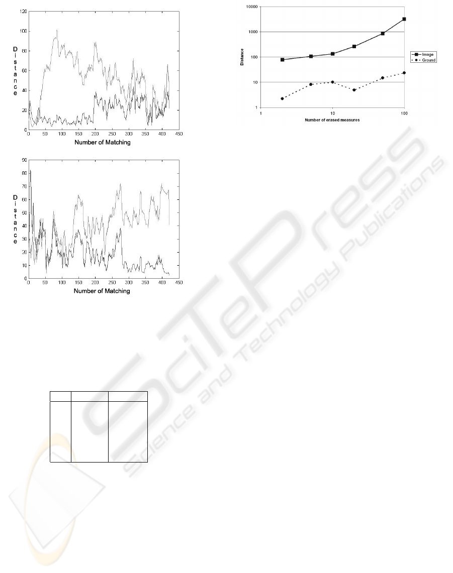
Figure 4: Distance between prediction and measure with

tracking on the ground (dark line) and tracking on the image

(light line). (a) Target moving away the camera (b) Target

moving to the camera.

Table 2: Mean distances in mm. between prediction and

measure applying different grades of decimation.

f Image Ground

1 54,9 18,89

2 78,49 22,89

3 97,75 26,58

5 132,01 31,06

8 180,02 40,33

12 248,08 55,93

Test 3: To test the precision of long-time predic-

tions, a determined number of consecutive measures

will be erased for both trackers. Also the same values

of Q and R are used. This test evaluates the possibil-

ity of recovering the object after an occlusion.

Different numbers of measures have been erased

in each test, from 2 to 100. To measure the accuracy

of each tracker, the distance in the ground between

the measure and the prediction after the erased block

of measures has been used. The results can be seen in

ﬁgure 5.

Here the differences between both trackers are

higher. The ground tracker does not lost the measure

Figure 5: Distances obtained after erased blocks of mea-

sures of different lengths (in logarithmic scale).

even after an occlusion of about 100 frames, main-

taining short distances between prediction and mea-

sure. However, the image tracker easily lost the mea-

sure after an occlusion of about 10 frames, giving very

bad predictions.

4.3 Using in Practice

Once tested the superiority of the ground tracker

in the laboratory, it has been conﬁrmed in real-life

videos of a football match . The test consists of a

video sequence, as the frame in ﬁgure 6.a, where two

football players are going to be tracked. Both play-

ers are running in parallel trajectories, but at different

distances from the camera. In this test, the necessity

of re-tuning of each trackers when trying to track dif-

ferent objects will be evaluated.

Both trackers will be conﬁgured with different

equivalent tunings for the distant player. Using the

homography, we can determine the relationship be-

tween a pixel in the image and the scale of the ﬁeld

to tune both trackers in a equivalent way. The mea-

sure noise R is ﬁxed, deﬁned for the image tracker,

and translated using the homography matrix for the

ground tracker. This tuning will be used on the nearby

player to check its validity.

The results can be seen on ﬁgure 7. As the two

trajectories are not equivalent, and may have differ-

ent accelerations and noises, the results cannot be di-

rectly compared. In any case, the ﬁgure shows that the

number of matchings obtained for the distant player is

similar for the two trackers, while the ground tracker

obtains more matchings than the image tracker for the

nearby player using the same tuning.

Although the number of matchings always can be

increased with higher values of the the matrices R and

Q, the prediction error and the possibility of crossing

with other measures would increase as well. Hence,

the application for a ground tracker is more important

if multiple objects are attempted to be tracked.

ICINCO 2008 - International Conference on Informatics in Control, Automation and Robotics

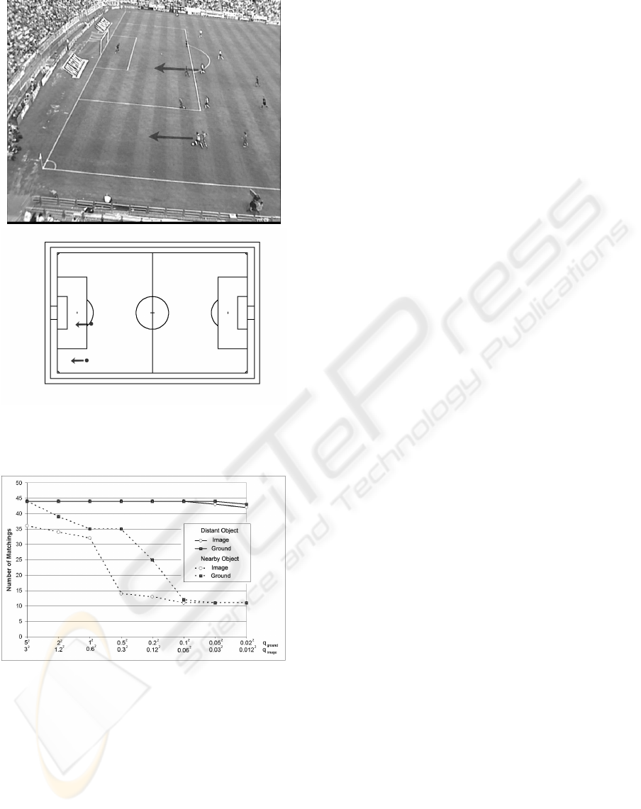
Figure 6: Frame of the video (up) and plane of the football

ﬁeld (down) of the video used. The arrows represent the

direction of the players that have been used for the test.

Figure 7: Number of matchings for different state noises.

The two scales are equivalent for the position of the distant

player.

5 CONCLUSIONS

In this paper we compared a tracker on the image

versus a tracker on the ground. A plane projective

transformation allows to make the tracking in real co-

ordinates which facilitates the tuning of the tracker,

gives measures in real coordinates and allows to re-

late different cameras in a common reference system.

Experimental results from laboratory test and from

real environments proved empirically that the tracker

on the ground achieves better results. We have also

shown some preliminary results for the automatic re-

calibration of the camera which avoids some of the

practical limitations of the approach. The continua-

tion of this work will be focused to the usage of mul-

tiple cameras, having the plane of the surroundings as

a common reference for the tracking.

ACKNOWLEDGEMENTS

This work was supported by project OTRI 2005/0388

”UZ - Real Zaragoza - DGA Collaboration Agree-

ment for development of a research project in the

sport performance improvement based on the image

analysis”, and it establishes the grounding for taking

real measures and statistics over the ground.

REFERENCES

A. Criminisi, I. R. and Zisserman, A. (September 1997).

A plane measuring device. In IEEE Transactions on

Pattern Analysis and Machine In Proc. BMVC, UK.

Bar-Shalom, T. and Fortmann, T. (1988). Tracking and

Data Association. Academic Press In.

Durucan, E. and Ebrahimi, T. (October 2001). Change de-

tection and background extraction by linear algebra.

In Proceedings of the IEEE, 89(10):1368-1381.

Fabrice Moscheni, S. B. and Kunt, M. (September 1998).

Spatiotemporal segmentation based on region merg-

ing. In IEEE Transactions on Pattern Analysis and

Machine Intelligence, 20(9):897-915.

Guerrero, J. and Sag

es, C. (2003). Robust line match-

ing and estimate of homographies simultaneously.

In IbPRIA, Pattern Recognition and Image Analysis,

LNCS 2652, 297–307.

Hartley, R. (1997). In defense of the eight-point algorithm.

In IEEE Trans. on Pattern Analysis and Machine In-

telligence, 19(6):580–593.

Hartley, R. and Zisserman, A. (2000). Multiple View Geom-

etry in Computer Vision. Cambridge University Press,

Cambridge.

Herrero, E., Orrite, C., and Senar, J. (2003). Detected

motion classiﬁcation with a double-background and a

neighborhood-based difference. In Pattern Recogni-

tion Letters, 24:2079-2092.

Isler, V., Khanna, S., Spletzer, J., and Taylor, C. J. (2005).

Target tracking with distributed sensors: The focus of

attention problem. In Computer Vision and Image Un-

derstanding, 100, 225-247.

Kalman, R. E. (1960). New approach to linear ﬁltering and

prediction problems. In Transactions of the ASME–

Journal of Basic Engineering, Volume 82, Series D,

35-45.

VISUAL TRACKING ON THE GROUND - A Comparative Analysis

Lee, L., Romano, R., and Stein, G. (August 2000). Mon-

itoring activities from multiple video streams: Estab-

lishing a common coordinate frame. In IEEE Trans-

actions on Pattern Analysis and Machine Intelligence,

22, n. 8.

Mundy, J. and Zisserman, A. (1992). Geometric Invariance

in Computer Vision. MIT Press, Boston.

Rousseeuw, P. and Leroy, A. (1987). Robust Regression and

Outlier Detection. John Wiley, New York.

Tissainayagam, P. and Suter, D. (2001). Visual tracking

with automatic motion model switching. In Pattern

Recognition, 34, 641-660.

ICINCO 2008 - International Conference on Informatics in Control, Automation and Robotics