
AN EXTENSION TO THE BEZIER SUB-DIVISION METHOD
TO COMPLETELY APPROXIMATE CURVES AND SURFACES
Andreas Savva, Vasso Stylianou and George Portides
Department of Computer Science, School of Sciences and Engineering, University of Nicosia
46 Makedonitissas Avenue, P.O. Box 24005, 1700 Nicosia, Cyprus
Keywords: Splines, Geometric modelling, Curves, Surfaces.
Abstract: Sub-division splines generate a number of new control points calculated fron the old control points. Both
control polygons/grids define the same curve/surface. At each iteration the resulting new points are much
greater in number than the old points and lie nearer to the actual curves. After a number of iterations, the
generated points lie on the actual curve, very close to each other, and by displaying them on a computer
screen the result is a smooth curve/surface. This paper describes a method, which is an extension to the
Bezier sub-division method, where the resulting curve is an approximation curve which interpolates only
the first and the last control points. The method is also derived for surfaces.
1 INTRODUCTION
The most popular methods for curve-fitting are
based on approximation – that is, the generated
curve passes near the original points approximating
their shape – like Bézier splines (Bezier, 1970,
1974, 1977), B-splines (Bartels et al, 1987), Beta-
splines (Barsky, 1981, 1986), ν-Spline (N
ielson,
1986), NURBS (Bartels et al, 1987; Piegl, 1990),
Kochanek spline (
Kochanek, 1984), Catmull-Rom
spline (Catmull and Rom, 1974) and many others.
Subdivision methods have also attracted a large
amount of research due to their ability to generated
complex surfaces defined by an arbitrary topology
of points, which are not based on a regular
rectangular mesh and even still today the most
important methods are those of Catmull and Clark
(Catmull and Clark, 1978) and Doo and Sabin (Doo
and Sabin, 1978).
This paper describes a subdivision method that
subdivides a Bézier curve and then generalizes it to
produce an approximated curve that interpolates
only the first and the last original points. Section 2
describes the Bezier sub-division method, section 3
derives its extension, and section 4 concludes.
2 THE BÉZIER SUBDIVISION
METHOD
The cubic Bézier curve defined by the control points
V
0
, V
1
, V
2
and V
3
is given by Eq.1 for
01≤≤u
.
3
3
2
2
2
1
3
0
)1(3)1(3)1()( uVuuVuuVuVuQ +−+−+−=
(1)
The same curve can also be generated by another
two Bezier curves,
(
)
2
u
Q
and
()
1
22
u
Q +
, where the
first is defined by the control points S
0
, S
1
, S
2
,
S
3
, and the second by T
0
, T
1
, T
2
, T
3
where S
3
=
T
0
, as illustrated in Fig.1. The control points S
0
, S
1
, S
2
, S
3
= T
0
, T
1
, T
2
, T
3
are called new points
and they can be calculated by the old points V
0
, V
1
,
V
2
and V
3
by Eq.1 and Eq.2 (Bartels et al, 1987).
The new points are twice as much as the original
points, (in-fact double minus one, since S
3
and T
0
is
the same point) and they lie nearer to the actual
curve than the original control polygon V
0
, V
1
, V
2
,
V
3
. Then from the new control points another set of
points (double minus one in size than the previous
points) can be calculated that are even nearer to the
actual curve. After a number of iterations the new
points lie on the actual curve, very close to each
other, and by displaying them on a computer screen
the result is a smooth curve.
143
Savva A., Stylianou V. and Portides G. (2008).
AN EXTENSION TO THE BEZIER SUB-DIVISION METHOD TO COMPLETELY APPROXIMATE CURVES AND SURFACES.
In Proceedings of the Third International Conference on Computer Graphics Theory and Applications, pages 143-146
DOI: 10.5220/0001099001430146
Copyright
c
SciTePress
()
()()
()
00
1
101
2
01 12
1
2012
4
01 23
12
1
30123
8
()
1
2
22 2
(+) (+)
()
1
33 +2 +
42 2 2
SV
SVV
VV VV
SVVV
VV VV
VV
SVVVV
⎫
=
⎪
⎪
⎪
⎪
=+
⎪
⎪
⎬
++⎛⎞
⎪
=++= +
⎜⎟
⎪
⎝⎠
⎪
⎪
+
⎛⎞
=+++=
⎪
⎜⎟
⎝⎠
⎪
⎭
(2)
()
()
()()
01 23
12
1
00123
8
12 23
1
1123
4
1
223
2
33
(+) (+)
()
1
33 +2 +
42 2 2
1
2
22 2
()
VV VV
VV
TVVVV
VV VV
TVVV
TVV
TV
⎫
+
⎛⎞
=+++=
⎪
⎜⎟
⎝⎠
⎪
⎪
++⎛⎞
⎪
=++= +
⎜⎟
⎪
⎝⎠⎪
⎬
⎪
=+
⎪
⎪
⎪
=
⎪
⎪
⎭
(3)
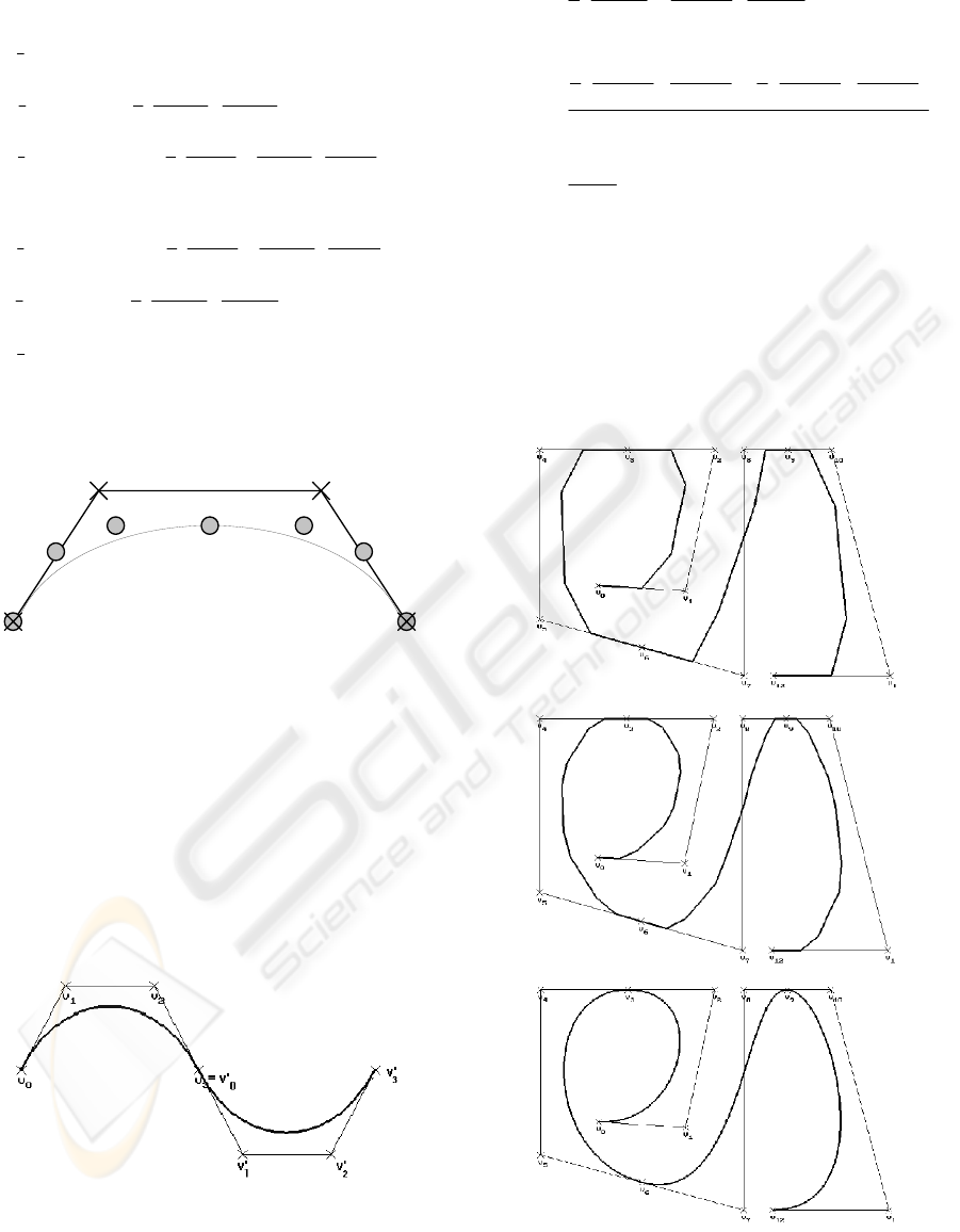
V
1
V
2
V
0
= S
0
S
1
S
2
T
1
T
2
= VT
33
S
30
= T
Figure1: The old and new points.
Consecutive segments in a composite Bézier
curve are C
1
continuous if the penultimate control
vertex of the first curve, the shared endpoint and the
second vertex of the next curve are collinear and
equally spaced. In Fig.2 the unprimed vertices
define one curve segment and the primed vertices
define another. Because V
2
, V
3
=
′
V
0
and
′
V
1
are
collinear and | V
3
- V
2
|=|
′
V
1
-
′
V
0
| the composite
curve will be C
1
continuous.
Figure2: Two Bézier segments.
From Eq.1 and Eq.2 it yields
()()()()
01 23
12
30
01 12 01 12
21
(+) (+)
1()
+2 +
42 2 2
11
22 2 22 2
2
2
(4)
VV VV
VV
ST
VV VV VV VV
ST
+
⎛⎞
==
⎜⎟
⎝⎠
++ ++
⎛⎞⎛⎞
++ +
⎜⎟⎜⎟
⎝⎠⎝⎠
=
+
=
which means that S
3
(which is the same point as T
0
)
is the midpoint of S
2
and T
1
and therefore the
required condition for continuity between successive
Bézier segments at each step is satisfied. Fig.3
illustrates a Bezier curve after 1, 2 and 6
subdivisions. It can be noted that the actual curve
interpolates the first and fourth control point of each
segment.
Figure 3: A recursive Bézier curve after 1, 2 and 6
subdivisions.
GRAPP 2008 - International Conference on Computer Graphics Theory and Applications
144
3 GENERATING AN
APPROXIMATION CURVE
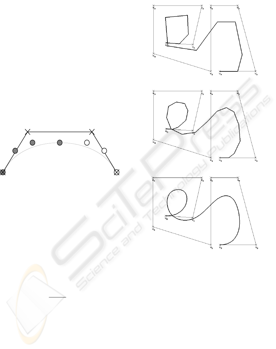
The new points can be divided into four different
categories (Fig.4). The V-points which correspond to
an old point at the two ends of the segment and are
equal to the old point, the V’-points which also
correspond to an old edge but not at the ends of the
segment, the E-points that correspond to an old edge
that one of the old points sharing the edge is at the
ends of the segment, and the E’-points that
corresponds to an old edge that none of the two old
vertices sharing the edge is at the ends of the
segment. Additionally, it can be emphasized that the
E’-points lie on the actual curve.
V
1
V
2
V' V'
EE
V
0
= V V
3
V =
E'
Figure 4: The new control polygon resulted from the
original one after one iteration.
It has been derived in (Savva and Clapworthy,
1998) that if we use V’-points and E’-points
everywhere on a curve except at the corner points
then the resulting curve becomes an approximation
curve that interpolates only the first and the last
control points. Also the penultimate control vertex
of the each previous segment, the shared endpoint
and the second vertex of the next segment does not
need to be collinear and equally spaced for
continuity, and actually the resulting curve is has C
2
continuity everywhere. This is illustrated in Fig.5.
Eq.4 shows that
21
3
2
ST
S
+
=
. This condition is
satisfied after the first iteration. But if we add the
midpoints of all the edges in the initial control
polygon then the resulting curve is similar as above
(Fig.5) but it gives a better approximation to the
control points as shown in Fig.6.
The same method is also derived for surfaces.
The resulting surface is an approximation to the
control grid but interpolates the corner points of the
surface.
Figure 5: An approximated curve that interpolates the first
and last control points after 1, 2 and 6 sub-divisions.
4 CONCLUSIONS
A Bezier curve interpolates the first and last control
point for each segment and in order to achieve C
1
continuity between successive segments the
penultimate control vertex of the first segment, the
shared endpoint and the second vertex of the next
curve must be collinear and equally spaced. Despite
the fact that there is only C
1
continuity at these
points, having to make the three control points
collinear makes it difficult to be used in modelling
applications.
AN EXTENSION TO THE BEZIER SUB-DIVISION METHOD TO COMPLETELY APPROXIMATE CURVES AND
SURFACES
145
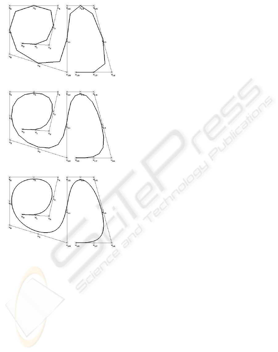
Figure 6: Adding the edge midpoints after 1, 2 and 6
subdivisions.
This paper describes an extension to the Bezier
sub-division scheme. The resulting curve is an
approximation curve that interpolates only the first
and the last control points and the curve has C2
continuity everywhere.
REFERENCES
Bartels R, Beatty J, Barsky B, An introduction to splines
for use in computer graphics & geometric modelling,
Morgan Kaufmann Publishers Inc., Los Altos,
California 94022, 1987
Barsky BA, The Beta-spline: A local representation based
on shape parameters and fundamental geometric
measures, PhD dissertation, Department of Computer
Science, University of Utah, 1981
Barsky BA, The Beta-spline: A curve and surface
representation for computer graphics and Computer
Aided Geometric Design, In: International Summer
Institute, Stirling, Scotland, R.A. Earnshaw and D.F.
Rogers (ed), Springer-Verlag, New York, 1986
Bézier PE, Emploi des machines à commande numérique,
Masson et Cie, Paris (translated by A. Robin Forrest
and Anne F. Pankhurst (1972) as "Numerical control -
Mathematics and applications", John Wiley & Sons
New York), 1970
Bézier PE, Mathematical and practical possibilities of
UNISURF, in Computer Aided Geometric Design,
Robert E. Barnhill & Richard F. Riesenfeld (ed),
Academic Press, New York, pp 127-152, 1974
Bézier PE, Essai de définition numérique des courbes et
des surfaces expérimentales, PhD dissertation,
l'Université Pierre et Marie Curie, Paris, 1977
Catmull EE, Clark JH, Recursively generated B-spline
surfaces on arbitrary topological meshes, Computer
Aided Design, 10(6):350-355, 1978
Catmull EE, Rom RJ, A class of local interpolating
splines, Computer Aided Geometric Design, Robert E.
Barnhill and Richard F. Riesenfeld (eds), Academic
Press, New York, 317-326, 1974
Doo D, Sabin M, Behaviour of recursive division surfaces
near extraordinary points, Computer Aided Design,
10(6):356-360, 1978
Kochanek DHU, Bartels RH, "Interpolating splines with
local tension, continuity and bias control", Computer
Graphics - SIGGRAPH '84 Conference Proceedings,
18(3):33-41, 1984
Nielson GM, Rectangular
ν
-splines, IEEE Computer
Graphics and Applications, 6(2), February, 35-40
(special issue on Parametric Curves and Surfaces),
1986
Piegl L, A toolbox for NURBS, Lecture notes, University
of South Florida, puplished in IEEE CG&A, 1990
Savva A, G.J. Clapworthy, A recursive approach to
parametric surfaces containing non-rectangular
patches, Proc International Conference on Information
Visualisation (IV’98), IEEE Press, London, pp 300-
306, July 1998.
GRAPP 2008 - International Conference on Computer Graphics Theory and Applications
146
