
A FULLY GPU-IMPLEMENTED RIGID BODY SIMULATOR
Álvaro del Monte, Roberto Torres, Pedro J. Martín and Antonio Gavilanes
Dpto. Sistemas Informáticos y Computación, Universidad Complutense de Madrid, Spain
Keywords: Physically based animations, Graphics Processing Units.
Abstract: In this paper we study how to implement a fully GPU-based rigid body simulator by programming shaders
for every phase of the simulation. We analyze the pros and cons of different approaches, and point out the
bottlenecks we have detected. We also apply the developed techniques to two case studies, comparing them
with the analogous versions running on CPU.
1 INTRODUCTION
The study of animation techniques has played a
decisive role in the evolution of computer graphics.
Traditionally in this topic, the issue of the physically
based motion of rigid bodies has been one of the
most attractive areas, mainly due to the high level of
realism achieved when rendering the involved
scenes. Since precision usually competes against the
run-time cost, most rigid body simulators have
specialized in configurations that get a trade-off
between accuracy and efficiency. However, it is
common to most of them to implement two phases
to solve two tasks: collision detection and collision
response. The first one looks for contacts between
pairs of objects, and it is usually split in other two
phases: the broad phase and the narrow phase. The
broad phase applies bounding volumes to objects in
order to check whether bounding volumes collide or
not (Teschner et al., 2005). If a pair collides, the
narrow phase determines if the included objects are
in collision. Only after determining that there will be
a real collision, the collision points are calculated.
The reason to decompose collision detection in these
two phases is that broad phase algorithms have a
much lower cost than those involved in the narrow
phase. Apart from these software solutions, there are
also other collision detection approaches which use
specific hardware (Raabe et al., 2006).
Different techniques have been proposed to deal
with the collision response. Although some
implementations allow interpenetration of objects,
such as the penalty method (McKenna and Zeltzer,
1990), most of them try to avoid it by accurately
computing the instant the impact comes up. This can
be achieved with the classic bisection method
(Baraff, 1997): the interval in which the collision
takes place is gradually reduced by comings and
goings in time. Once the collision instant is
computed, the response can be obtained by applying
the forces which solve certain constraints −Baraff’s
constraint method (Baraff, 1989)− or by
instantaneously modifying the velocity of the objects
after computing the related impulse (Mirtich, 1996).
The efficiency of a rigid body simulator does not
only depend on the components integrating the
system, but also on the way they are integrated into
the simulation loop, especially when a large number
of objects are involved. Note that the collision time
of a pair of objects can affect to –even avoid– many
other collisions that come up later in the same loop
iteration. For this reason, the computation of the
instant for these other collisions is a useless task that
could collapse the simulation as a whole. In order to
prevent this eventuality, in a uniprocessor context,
(Mirtich, 2000) proposed the timewarp algorithm
which uses heaps as data structures.
On other hand, the evolution of GPUs, as regards
performance and programmability, has brought
about their intensive use in many applications.
Today they are a key element in the design stage of
any simulator. This is the case for the interactive
visualization of particle systems (Krüger et al.,
2005), where GPUs have been used to parallelly
manage the independent movement of each particle.
In the context of rigid body simulations, shaders
have been used to relieve CPU of specific tasks, but
never to solve the whole algorithm. For instance
(Yuksel, 2007) introduces fragment shaders in the
rendering phase to quickly support special effects,
342
del Monte Á., Torres R., J. Martín P. and Gavilanes A. (2008).
A FULLY GPU-IMPLEMENTED RIGID BODY SIMULATOR.
In Proceedings of the Third International Conference on Computer Graphics Theory and Applications, pages 342-350
DOI: 10.5220/0001098503420350
Copyright
c
SciTePress

while all the computations involved in the
simulation part are implemented on the CPU.
Concerning the simulation methodology, moving the
detection of collisions to GPU has been the most
studied topic. Collision detection algorithms on
GPUs can be classified into two categories. On one
hand, screen-space approaches use the depth or
stencil buffers to perform the collision tests by
rendering the geometry primitives (Govindaraju et
al., 2005) (Teschner et al., 2005). Their main
problems are that effectiveness is often limited by
the image space resolution, and that only potentially
colliding pairs are reported, so another test must be
applied on the CPU later.
On the other hand, object-space approaches use
the floating point bandwidth and programmability of
modern GPUs to implement the collision test.
(Zhang and Kim, 2007) performs massively-parallel
pairwise, overlapping tests onto AABB streams,
although exact primitive-level intersection tests are
performed on CPU. (Greβ and Zachmann, 2004)
(Horn, 2005) (Greβ et al., 2006) generate bounding
volume hierarchies on the GPU from a geometry
imaged (Gu et al., 2002) representation of the solids.
In order to expose the parallel processing
capabilities of the GPU, they breadth-first traverse
these hierarchies by using the non-uniform stream
reduction presented in (Horn, 2005). Nevertheless,
these approaches cannot autonomously operate on
the GPU, since the selection of the objects of the
pair to be tested is usually chosen on the CPU.
Furthermore, they do not apply any response when
the objects actually collide, so they should require
extra CPU collaboration to address interactions.
In the context of deformable objects, recent
papers have used the GPU capabilities to quickly
update their geometry: (Pascale et al., 2005)
proposes the use of vertex shaders to locally deform
the object, (Zhang and Kim, 2007) employs a
fragment shader to update the AABB streams, and
(Kim et al., 2006) uses a fragment shader to compute
the mass properties of rigid bodies in a buoyancy
simulation. Nevertheless, none of these papers cover
interactions between objects.
In this paper we study how to implement a fully
GPU-based rigid body simulator, by programming
shaders for every phase of the simulation. We
analyze the pros and cons of different approaches,
and point out the bottlenecks we have detected. We
also apply the developed techniques to two case
studies, comparing them with the analogous versions
running on CPU.
2 THE SIMULATION LOOP
The animation in a rigid body simulation is achieved
through a main loop, which updates the information
related to every object, after a cycle or step has been
completed. The size of the step must be accurately
chosen because of stability reasons. So the realism
level of the simulation directly depends on it.
In order to complete a step, the dynamics of
every object (position of its center of mass
x(t),
orientation
r(t), linear velocity v(t), and angular
velocity ω(t)) must be updated by using numerical
methods to solve ordinary differential equations.
Figure 1 shows both the configuration
Y(t) of the
state of an object and its time derivative in a 2D
scenario. In this case, the vector
r(t) and ω(t)
can be simplified to single scalars. Velocities change
according to the action of forces, since there exist
simple relations between their time derivatives and
the applied forces. The torque generated by a force
F(t) is defined as τ(t) = (p-x(t))×F(t),
where p is the location at where F(t) acts. Again
the vector
τ(t) can be simplified to a single scalar
in a 2D scenario. The mass M and the moment of
inertia
I are two scalars expressing the resistance of
a body to a linear or an angular motion, respectively.
The collision computation is the main task
involved in each step, since collisions make forces
generate motion. It is made up the three sequential
stages that will be presented in the following
subsections. Roughly speaking, rigid body
simulation can be considered as a large catalogue of
subroutines, some of those are carefully chosen to
fill each of these stages to build systems that
efficiently solve the specific scenes they drive. Here
we show how some of these subroutines can be
implemented on GPU, analyzing pros and cons with
respect to other approaches. Since the subroutines
can be independently incorporated into the whole
simulator, they are interchangeable parts; therefore
systems alternating CPU- and GPU-computations
are available. Nevertheless such hybrid simulators
would require additional tasks to change the
processor (e.g. transmitting data between CPU and
GPU, binding textures to shaders, and assigning
values to uniform variables) that could slow down
the simulation. Thus we will only consider fully
GPU-implementations in the sequel.
A FULLY GPU-IMPLEMENTED RIGID BODY SIMULATOR
343

⎟
⎟
⎟
⎟
⎟
⎠
⎞
⎜
⎜
⎜
⎜
⎜
⎝
⎛
=
⎟
⎟
⎟
⎟
⎟
⎠
⎞
⎜
⎜
⎜
⎜
⎜
⎝
⎛
=
It
MtF
t
tv
dt
tdY
t
tv
tr
tx
tY
)(
)(
)(
)(
)(
)(
)(
)(
)(
)(
τ
ω
ω
Figure 1: Configuration of the state of an object and its.
The programming of GPUs includes stream
processing which is based on the definition of
kernels and streams. Kernels process data in parallel,
while streams organize the information in the
memory card. In our GPU-implementations we use
the following three textures of size
2
n
x1 –where 2
n
is the chosen number of objects; we use power-of-
two sizes since they are required for the algorithm of
Section 2.2– to store the state of any object:
Linear: a RGBA-texture to store
x(t) and
v(t)
Rotational: a RGBA-texture to store
r(t) and
ω(t)
Geometry: a RGBA-texture to store the
geometry of any object as follows: component
R holds the index of the first vertex of the
object, component G is the number of its
vertices, component B keeps its mass, and
component A stores its moment of inertia.
The dynamics of an object is updated after every
simulation step, so the two first textures act as input
and output at the same time, thus we use the ping-
pong technique described in (Gödekke, 2005). Note
that although only two components of the Rotational
texture are required, the format RGBA has been
chosen to allow the renderization to it. The
Geometry texture can be seen as globally-shared
read-only memory that always acts as input. It is
used to determine the current coordinates of the
vertices of the objects, which will be used in the
following stages. We use the first two components
of its texels to access the real coordinates of the
vertices, which will be in a fourth texture called
Vertices. This one can also be seen as globally-
shared read-only memory to keep the –locally
expressed– coordinates. In a 2D scenario, the format
RGBA stores the coordinates of two vertices in each
texel, so the size can be reduced to
Σ{⎡vertex
i
/2⎤
/ 0≤i≤2
n
-1}. The following is a fragment of the
GLSL-code to access the vertices of an object. This
is graphically shown in Figure 2.
//We extract the geometry data of objectI
vec4 geo=textureRect(Geometry,vec2(objectI,0.5));
//The x-component of geo is the address of
//the first vertex of objectI in Vertices
float index=geo.x+0.5;
//We extract the first two vertices of objectI
vec2 v1=textureRect(Vertices,vec2(index,0.5)).xy;
vec2 v2=textureRect(Vertices,vec2(index,0.5)).zw;
In order to focus on the GPU-implementation issues,
we have chosen a 2D rather than a 3D scenario.
Extending the algorithms we propose to the 3D case
is a technical exercise, not covered by this paper. In
this case, most of the data we manage would become
larger, so additional textures would be required. For
example,
x(t) and v(t) should be stored in
separated textures, since they are 3D vectors.
Angular data as
ω(t) and τ(t) also become 3D
vectors, while
r(t) and I should be implemented
through quaternions and 3×3 matrices, respectively.
2.1 Detecting Collisions
In the collision detection stage, the simulator looks
for contacts between pairs of objects. The realism of
the simulation strongly relies on the accuracy in the
detection and computation of these collisions. In
order to minimize the computational effort to detect
collisions, each object is wrapped with an axis
aligned bounding box (AABB). The premise that
motivates its use is the fact that intersections among
AABBs are much easier to detect than the collisions
between the actual objects.
In the simulation loop, prior to compute AABBs
intersections, each volume must be updated
depending on the current position of the contained
object. There are two ways to envelop the object
within a new AABB: either by using the vertices of
the updated object or by using the vertices of the
updated AABB. We have chosen the first method,
which has an updating cost obviously greater than
the second one, but more no-collision situations are
discarded since the volume is tighter to its object.
In order to update bounding volumes, we require
one pass of the kernel
UpdateAABB which renders
Geometry
22, 6, 2, 5 25, 10, 2, 5
25 22
Vertices
Figure 2: Accessing the vertices of an object.
GRAPP 2008 - International Conference on Computer Graphics Theory and Applications
344

to a RGBA-texture of size
2
n
x1 to encode the
updated AABB related to any object. More
precisely, RG and BA are used for its left-bottom
and right-top corner, respectively. Each fragment
processing includes reading both the current position
and rotation of the object as well as mapping these
transformations to all of its vertices to build the
AABB. Thus, its inputs are the Linear, Rotational,
Geometry and Vertices textures. The cost of
fragment processing depends on the number of
vertices of the related object; hence the whole pass is
a linear operation w.r.t. the total number of vertices.
Once the AABBs have been updated, we check
for overlapping by using one pass of the kernel
OverlapAABB. Its input is the output of the previous
kernel. It renders to a Luminance texture of size
2
n
X2
n
, where the texel (i,j) indicates whether the
AABBs of objects
i and j get to be overlapped.
Now, the cost of a fragment processing is constant,
since only one comparison of the involved corners is
required. Moreover the symmetry of the texture can
be used to restrict the computation to the lower
triangular (LT) region below its main diagonal.
The next phase consists in determining if the
objects contained in the overlapping AABBs
actually collide. We detect such collisions, and the
related collision times, on GPU. In the case of
convex polygons, specific algorithms have been
designed to check whether two objects collide. We
think the classic approach based on separating
planes is not convenient for a GPU implementation,
since they seem rather difficult to be reused in the
simulation. Instead we use a simple algorithm which
behaves well in almost every situation; we do not
consider the remaining ones to be a problem since
the paper does not focus on the simulation realism,
but on comparing GPU- to CPU-implementations.
We actually test if every vertex of a given polygon is
inside the other one. This naive algorithm could be
improved by using the O’Rourke’s approach
(O’Rourke, 1993).
For every pair of objects that will collide after a
complete step, we use the method of bisection to
calculate the exact collision time by testing whether
the objects collide each other in the middle of the
current interval of time. Since the first iteration of
this loop requires the texture produced by
OverlapAABB, the bisection method has been
divided into two kernels:
Bisection1 and
Bisection2. Nevertheless, the two kernels are
essentially the same. They share the Linear,
Rotational, Geometry and Vertices textures as
inputs, and they render to a RGBA-texture
HitTimes of size
2
n
X2
n
, where each texel stores four
data corresponding to the involved pair of objects:
the bounds of the interval enclosing the collision, a
flag to continue (0) or to reject (1) the search of
collision, and the hit time. In order to integrate the
loop related to
Bisection2 we have implemented
two while-sentences. The first one occurs inside the
shader and it is used to calculate the hit time. In
order to prevent from the execution of too many
iterations, we use an extra parameter -a uniform
variable
iter- to control the number of iterations,
since the number of instructions available on the
card is limited. The second one is outside the shader
and it is used to execute the kernel several times.
Due to this multi-pass approach, we successively use
outputs as next inputs. Programming this way allows
us to compare different combinations. The following
is a fragment of the GLSL-pseudo-code of the
Bisection kernels. The uniform variable epsilon
is the accuracy when determining the hit time.
uniform samplerRect Linear, Rotational,
Geometry, Vertices, HitTimes;
uniform float epsilon;
uniform int iter;
vec4 Bisection(float coordObject1, float
coordObject2, float maxTime, float minTime){
//[minTime,maxTime] is the current interval
float maxT=maxTime; float minT=minTime;
vec4 result;
int i=0;
while((maxT-minT>epsilon) && (i<iter)){
float midT=(maxT+minT)/2.0;
if (collision in midT) maxT=midT;
else minT=midT;
i++;
}
if (maxT-minT<=epsilon)
result=vec4(minT,maxT,1,minT);//bisection ends
else result=vec4(minT,maxT,0,minT);//[minT,maxT]
//is the interval for the next bisection pass
return result;
} //Bisection
Table 1 shows timing data for two cases. In the
column Inside (
iter=ceil(-log2(epsilon))),
every iteration takes place inside the shader, while in
the column Outside (
iter=1) only one takes place
inside the kernel. As we see, executing the loop
inside the shader is much better than a pure multi-
pass approach. Along this paper, we have tested the
GPU implementations on a NVIDIA GeForce 7900
GS card. All timing data will be always expressed in
seconds along the paper.
A FULLY GPU-IMPLEMENTED RIGID BODY SIMULATOR
345
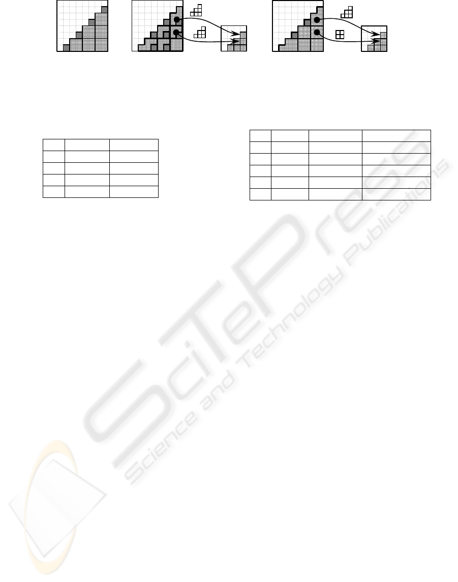
Figure 3: a) Darkest texels are not visited when the classic minimization method is applied to the LT region. b) 6-reduction.
c) (4+6)-reduction. In b) and c), darkest texels are visited more than once.
Table 1: Running 1000 times the Bisection kernels for the
two forms of iterating. An initial random scene has been
used in each row.
At the end of the two kernels we have a texture
of size
2
n
X2
n
, with the alpha component containing
the hit time t∈[0,1] for every pair of objects, or a
constant greater than 1 to indicate that the related
objects do not collide. Due to symmetry, the kernel
only requires to process the LT region of the texture.
2.2 Searching the First Collision
There are different ways to process the contacts
computed in the previous phase. On one hand, we
can arrange the contacts with respect to the collision
time. The problem is that solving one collision may
affect many other collisions produced later within
the same step. To be precise, some of them could not
be produced or even new collisions could arise. On
the other hand, there is a simpler approach
consisting in truncating the step at the just moment
of the first contact, and discarding the rest. We have
chosen this latter approach; so we have used the
classic reduction kernel (Buck and Purcell, 2004) to
compute the minimum of the collision times.
Nevertheless, we have proposed and analyzed
different methods to improve the classic reduction
kernel by exploiting the symmetry of the input
textures. For all of them, the input is a texture of size
2
n
X2
n
, where the texel (i,j) stores the floating
point corresponding to the collision time of the
objects
i and j, or a constant greater than 1 if they
do not collide. Since the texture is symmetric and its
main diagonal is irrelevant, we can restrict to texels
with
i<j. The output of the kernel will be computed
by successively iterating a shader to halve each
texture dimension.
In the classic method, the fragment processing
computes the minimum of a
2×2 square. Since the
texture is symmetric, our approach only requires
Table 2: Comparing the three reduction methods for 1000
complete minimizations.
processing the LT region. If we applied the classic
2×2 reduction to the LT region, some texels would
not be considered (Figure 3a). In order to include
them, we must visit six texels when processing
fragment
(i,j), those with coordinates (2i,2j),
(2i+1,2j), (2i,2j+1), (2i+1,2j+1), (2i-
1,2j) and (2i+1,2j+2). This solution, which we
call 6-reduction, improves the classic algorithm, but
it generates too many redundant readings (Figure
3b). In order to avoid them, we exploit the fact that
only the adjacent components to the diagonal need
to check the six elements, while the others only
require the four elements of the classic method.
Therefore this (4+6)-reduction is a combination of
two shaders: one to check the six elements that
correspond to fragments adjacent to the diagonal,
and the other one to check the four elements that
correspond to the remaining fragments of the LT
region (Figure 3c).
The complexity of a pass reducing a texture of
size
2m×2m to a texture of size m×m is 4m
2
for the
classic algorithm,
3(m
2
-m) for the 6-reduction and
2(m
2
-1) for the (4+6)-reduction, with respect to the
number of required readings. Since the complete
reduction process is based on a multi-pass approach,
the quadratic coefficient involved in a single pass
becomes critical. Table 2 compares the three
options, running 1000 complete minimizations. As it
was expected, results report that the (4+6)-reduction
significantly reduces time as the texture size
increases.
2.3 Solving the First Collision
After computing the minimum hit time, we must
apply the related response on the GPU. Firstly, we
2
n
Inside Outside
2
8
0.6100 1.1500
2
9
0.7200 1.7875
2
10
0.7600 10.200
2
11
1.1400 10.600
2
n
Classic 6-reduction (4+6)-reduction
2
8
1.422 1.625 1.532
2
9
1.750 1.906 1.438
2
10
2.031 2.047 1.656
2
11
3.187 2.437 1.831
2
12
14.265 10.939 6.484
a)
b
)
c)
GRAPP 2008 - International Conference on Computer Graphics Theory and Applications
346
check whether the contacts at the same time are real
collisions. The relative velocity
V
rel
of the pair of
objects A and B is useful to solve this question:
( ..)()( (..)1)
AB
rel hit hit hit
dp dp
Vttnt
dt dt
⎛⎞
=−⋅
⎜⎟
⎝⎠
where
dp/dt denotes the velocity of the contact
point within the corresponding object, and
n is the
contact normal. If V
rel
<0 (see Figure 4), the objects
are colliding and an impulse must be computed to
avoid that they get overlapped. The impulse
J is an
instantaneous force, thus it produces a variation of
the velocities according to the following equations:
Δv=J/M and Δω =Γ
J
/I, where the torque is defined
by Γ
J
=(p-x(t))×J. The impulse J is a vector
whose direction is the contact normal n and whose
magnitude
j must be computed by using the
following equation (2):
00
00
(1 )
() ()
11
() ()
rel
AB
A
B
AB A B
V
j
rnt rnt
nt r nt r
MM I I
ε
−
−+
=
⎛⎞ ⎛⎞
××
++ ×+ ×
⎜⎟ ⎜⎟
⎝⎠ ⎝⎠
where
ε is the restitution coefficient between the two
objects,
V
rel
−
is the relative velocity before the
impulse, and
r
A
, r
B
are the vectors from the center of
mass of each object to the contact point p. The
action of
J is positive (+jn(t)) on the object A and
negative (
-jn(t)) on B.
The computation of the impulse is carried out by
the kernel
Impulse. Its inputs are the Linear,
Rotational, Geometry, Vertices and HitTimes
textures, and the minimum hit time. It renders to a
RGBA-texture of size
2
n
X2
n
, where the texel (i,j)
stores the accumulation of the impulses between the
objects
i and j, since several collisions points can
simultaneously arise. The impulse is computed
whenever the collision time equals the minimum hit
time. If this is the case, the accumulation of impulses
is performed as the following pseudo-code shows.
while (i<numVerticesA) {
while (j<numEdgesB) {
if (i-th vertex of A is on the j-th edge of B){
1.- Compute Vrel of A and B in the i-th
vertex of A
2.- If (Vrel<0) {
2.1.- Compute the impulse
2.2.- Accumulate the impulse
}}}}
//Repeat with vertices of B and edges of A
Finally we execute one pass of any of the
following kernels to update the scene after a step of
the simulation:
NoCollisionForward and
CollisionForward. Their inputs and outputs are
the Linear and Rotational textures. The kernel
NoCollisionForward is used when the instant of
the first collision is greater than a step of time. In
this case, no collision is produced, the impulse is not
computed, and the kernel updates the objects until
the end of the step of time. Thus, processing a
fragment requires constant time. The kernel
CollisionForward is used otherwise and includes
the output texture of the kernel
Impulse as input.
This kernel accumulates the impulses between an
object and the remaining objects, and applies the
total impulse. Hence processing a fragment requires
linear time.
3 THE RENDERING PHASE
The image of the objects after a step is obtained by a
vertex shader, which applies the transformations
needed to suitably translate and rotate the object in
the scene. This entails two jobs.
First of all, the translation and the rotation of the
processed object must be loaded. Since the Linear
and Rotational textures are located in memory card,
they must be read back from GPU to CPU after any
step. This option is called toCPU in Table 3. On the
other hand, we can access these data within the
shader itself by using a uniform variable to hold the
texture coordinates that must be read. We use such a
variable as an index, which must be properly
assigned before rendering the object. This option is
called Index in Table 3. The total cost of the latter
approach includes two texture accesses per vertex,
plus an extra uniform assignment per object.
A
B
n
V
rel
V
rel
> 0
A
B
n
V
rel
V
rel
= 0
A
B
n
V
rel
V
rel
< 0
Figure 4: Relative velocity
(
)()( t
dt
dp
t
dt
dp
V
BA
rel
−=
) of objects A and B.
A FULLY GPU-IMPLEMENTED RIGID BODY SIMULATOR
347

Second, the shader needs the local coordinates of
every vertex. Now we must decide how to send
vertices to the pipeline. We propose these options:
1. Sending fictitious coordinates that will be
replaced with the coordinates stored in the
Vertices texture. In order to access the
Geometry and Vertices textures, the shader
needs the index of the object and the ordinal of
the vertex within the object. To this aim, the
simplest way is to use the fictitious coordinates
to communicate these data to the shader. More
precisely, the
x-coordinate indicates the object
and the
y-coordinate refers to the vertex offset
when accessing the Vertices texture. Hence any
fragment processing requires two texture
accesses: one to read the object data in the
Geometry texture, and another to get the local
coordinates of the vertex in the Vertices texture.
2. Sending fictitious coordinates and using one of
them to indicate the ordinal of the vertex within
the object, as in the previous option, and the
other one to refer to the location of the first
vertex of the object within the Vertices texture.
Thus, we save one access per vertex.
3. Directly sending the local coordinates of each
vertex to save the two accesses. The
disadvantage of this option is that a copy of the
Vertices texture must be located in CPU
memory.
Table 3 compares the six combinations related to the
solutions of the two jobs, that is, the two options to
read the transformations and the three options to
send the coordinates to the pipeline. The time
measures correspond to 1000 renderings of a random
scene configuration. In the last row we show how
many texture accesses (a) are required per vertex,
how many uniforms (u) must be assigned per object,
and how many textures (t) have to be read from
GPU to CPU. Note that texture accesses from vertex
shaders are only available from shader model 3.0.
Table 3: Comparing the six implementations of the
rendering phase.
4 CASE STUDIES
We have implemented two versions of the previous
simulation algorithms, including different geometric
shapes: the first for circles and the second for
convex polygons. Our shaders need several GPU
capabilities supported from the shader model 3.0,
such as texture accesses from a vertex shader, or
conditions in loops that cannot be solved at compile
time. The time measures correspond to 1000 steps in
order to reduce measurement errors. Apart from the
GPU implementation, we have also developed a
CPU version of every algorithm. They have been run
on an Intel Core 2 Duo 1,86 Ghz. A comparison is
shown in Table 4. The initial scene is randomly
generated. In addition, initial positions are enclosed
within a squared room to improve the simulation
visualization. Walls are differently implemented in
each case.
4.1 Circles
Circles are the simplest shapes in rigid body
simulation, mainly because rotations can be skipped.
It is also possible to compute the hit time of two
circles algebraically, thus the bisection loop can be
changed into a constant time code. It is enough to
solve the equation
distance(A+ta,B+tb)=r
A
+r
B
,
where r
A
, r
B
are the radius, A, B are the centres, and
a, b are the linear velocities of the two circles. It
leads to a second order equation which must be
solved to find the, at the most, two values of
t.
Nevertheless the difference between both
approaches is irrelevant since the few but expensive
computations of the algebraic approach can be
compared to the low-cost but many iterations of the
bisection loop. Table 4 compares both approaches.
The walls are also easy to implement since perfect
reflections are applied.
4.2 Convex Polygons
For the sake of convenience, we only generate
scenes with regular polygons. In fact we only use
triangles in Table 4. The bisection kernels are
required to compute hit times. Walls are
implemented as rectangular objects with infinite
mass, so they are static objects. Table 4 shows that
the GPU implementation significantly reduces time
as the number of objects increases.
Option 1 Option 2 Option 3
2
n
Index toCPU Index toCPU Index toCPU
2
8
16.659
9
16.659
9
16.649
9
16.649
9
16.659
9
16.659
9
2
9
25.909
9
26.239
9
25.870
0
23.969
9
16.670
0
16.659
9
2
10
51.580
0
49.110
0
50.910
0
45.639
9
33.330
0
16.659
9
2
11
117.26
0
102.27
9
102.37
9
89.750
0
65.529
9
16.659
9
4a
2a+2t+2
u
3a+1u
1a+2t+2
u
2a+1u 2t+2u
GRAPP 2008 - International Conference on Computer Graphics Theory and Applications
348
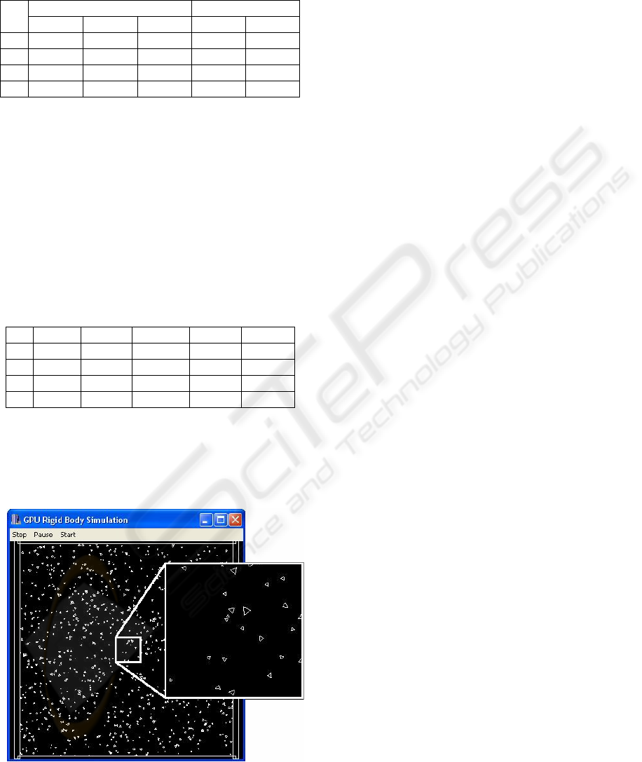
Table 4: Comparing the three circles implementations
(GPU-algebraic, GPU-bisection, CPU-bisection) and the
two polygons ones (GPU-bisection, CPU-bisection).
Table 5 shows the timing data of the main
kernels of the simulation algorithm after running
1000 steps on the same initial random configuration.
Hence we cannot use it to deduce which kernel is the
most demanding one, since their execution depends
on the initial configuration. For instance, the
Bisection2 kernel will not run whenever the
OverlapAABB kernel computed no pair of
overlapping AABBs, and the
Impulse and the
CollisionForward kernels do not run whenever
no collision arises.
Table 5: Timing data of the kernels used in the simulation.
Finally, we show in Figure 5 a snapshot of the
rigid body simulator applied to a scene made up of
1024 dynamic triangles, with a detail of the scene
highlighted.
Figure 5: Snapshot of the rigid body simulator.
5 CONCLUSIONS
In this paper we have presented a fully GPU-
implemented rigid body simulator, which is suitably
composed of different −fragment and vertex−
shaders to execute both the simulation and the
renderization tasks. Moreover we have proposed
several solutions for many of the development
phases, comparing their behavior. Finally, we have
applied these techniques to two case studies, one
based on circles and another on convex polygons.
The main contribution of the paper is to show
that the GPU capabilities can be used to improve the
overall timing of a CPU implementation. In the case
studies, we compare our GPU solutions to analogous
CPU versions, showing that GPU implementations
win as the number of objects increases.
REFERENCES
Baraff, D., 1989. Analytical Methods for Dynamic
Simulation of Non-Penetrating Rigid Bodies. In
SIGGRAPH’89, 223-232.
Baraff, D., 1997. Rigid Body Simulation. An Introduction
to Physically Based Modeling. In SIGGRAPH’97,
course notes.
Buck, I., Purcell, T., 2004. A Toolkit for Computation on
GPUs. In GPU Gems, Addison-Wesley, 621-636.
Göddeke, D., 2005. GPGPU: Basic Math Tutorial. TR.
300, Fachbereich Mathematik, Universität Dortmund.
Govindaraju, N., Lin, M., Manocha, D., 2005. Quick-
CULLIDE: Fast Inter- and Intra-Object Collision
Culling Using Graphics Hardware. In IEEE Virtual
Reality Conference, 59-66, 319.
Greß, A., Guthe, M., Klein, R., 2006. GPU-based
Collision Detection for Deformable Parameterized
Surfaces. In Computer Graphics Forum 25(3), 497-506.
Greß, A., Zachmann, G., 2004. Object-Space Interference
Detection on Programmable Graphics Hardware. In
Geometric Modeling and Computation. Proc. of
SIAM Conference on Geometric Design and
Computing, 311-328.
Gu, X., Gortler, S., Hoppe, H., 2002. Geometry Images. In
ACM Trans. Graph 21(3), 355-361.
Horn, D., 2005. Stream reduction operations for GPGPU
applications. In GPU Gems 2, Addison-Wesley, 573-
589.
Kim, J., Kim, S., Ko, H., Terzopoulos, D., 2006. Fast GPU
Computation of the Mass Properties of a General
Shape and its Application to Bouyancy Simulation. In
Int. Journal of Computer Graphics 22(9), 856-864.
Krüger, J., Kipfer, P., Kondratieva, P., Westermann, R.,
2005. A Particle System for Interactive Visualization
of 3D Flows. In IEEE Transactions on Visualization
and Computer Graphics 11(6), 744-756.
Circles Polygons
2
n
GPU-alg GPU-bis CPU-bis GPU-bis CPU-bis
2
8
33.62 33.56 33.33 17.47 16.66
2
9
50.16 50.16 86.14 17.50 36.27
2
10
83.49 83.47 356.42 26.83 192.63
2
11
166.79 166.89 1603.10 67.62 810
2
n
Update Overlap Bisection Impulse Forward
2
8
0.1599 0.2500 0.6100 0.3200 0.0390
2
9
0.1700 0.6869 0.7200 0.3200 0.0799
2
10
0.1899 2.4700 0.7600 0.3600 0.2100
2
11
0.2300 9.4600 1.1400 0.5200 0.2300
A FULLY GPU-IMPLEMENTED RIGID BODY SIMULATOR
349

McKenna, M., Zeltzer, D., 1990. Dynamic Simulation of
Autonomous Legged Locomotion. In Computer
Graphics 24(4), 29-38.
Mirtich, B., 1996. Impulse-Based Dynamic Simulation of
Rigid Body Systems. Ph. D. dissertation. University of
California, Berkeley, CA.
Mirtich, B., 2000. Timewarp Rigid Body Simulation. In
SIGGRAPH‘00, 193-200.
O’Rourke, J., 1993. Computational Geometry in C,
Cambridge University Press.
Pascale, M., Sarcuni, G., Prattichizzo, D., 2005. Real-
Time Soft-Finger Grasping of Physically Based Quasi-
Rigid Objects. In World Haptic Conference, 545-546.
Raabe, A., Hochgürtel, S., Anlauf, J., Zachmann, G.,
2006. Hardware-Accelerated Collision Detection using
Bounded-Error Fixed-Point Arithmetic. In Journal of
WSCG 14, 17-24.
Teschner, M., Kimmerle, S., Heidelberger, B., Zachmman,
G., Raghupathi, L., Furmann, A., Cani, M., Faure, F.,
Magnenat-Thalmann, N., Strasser, W., Volino, P.,
2005. Collision detection for deformable objects. In
Computer Graphics Forum 24(1), 61-81.
Yuksel, C., 2007. Real-Time Impulse-Based Rigid Body
Simulation and Rendering. Master Thesis, Texas
A&M University.
Zhang, X., Kim, Y. J., 2007. Interactive Collision
Detection for Deformable Models using Streaming
AABBs. In IEEE Trans. on Visualization and
Computer Graphics 13(2), 318-329.
GRAPP 2008 - International Conference on Computer Graphics Theory and Applications
350
