
ANALYSIS OF POINT CLOUDS
Using Conformal Geometric Algebra
Dietmar Hildenbrand
Research Center of Excellence for Computer Graphics, University of Technology, Darmstadt, Germany
Eckhard Hitzer
Department of Applied Physics, University of Fukui, Japan
Keywords:
Geometric algebra, geometric computing, point clouds, osculating circle, fitting of spheres, bounding spheres.
Abstract:
This paper presents some basics for the analysis of point clouds using the geometrically intuitive mathematical
framework of conformal geometric algebra. In this framework it is easy to compute with osculating circles
for the description of local curvature. Also methods for the fitting of spheres as well as bounding spheres are
presented. In a nutshell, this paper provides a starting point for shape analysis based on this new, geometrically
intuitive and promising technology.
1 INTRODUCTION
The main contribution of this paper is its collection
of properties and basic algorithms that make it a very
promising tool for the analysis of point clouds. Please
refer for instance to (Schnabel et al., 2007) for current
research results concerning this application.
Conformal geometric algebra has shown some ad-
vantages in recent years. It is very easy to calculate
directly with geometric objects like spheres, circles
and planes. Also transformations can be handled very
easily. This mathematical framework is able to unify
a lot of mathematical systems like vector algebra, pro-
jective geometry, quaternions or Pl¨ucker coordinates.
While geometric algebra formerly had the prob-
lem of efficiency, now there are approaches available
so that algorithms written in this framework can even
be faster than conventional algorithms (see (Hilden-
brand et al., 2006)).
Like implementations of quaternions can be
more robust than rotation matrices geometric algebra
promises to deliver more robust algorithms. As an ex-
ample, planes can be represented as specific spheres
allowing to fit spheres or planes into point sets (see
(Hildenbrand, 2005)).
2 FOUNDATIONS OF
CONFORMAL GEOMETRIC
ALGEBRA
Blades are the basic computational elements and the
basic geometric entities of the geometric algebra. For
example, the 5D Conformal Geometric Algebra pro-
vides a great variety of basic geometric entities to
compute with. It consists of blades with grades 0, 1,
2, 3, 4 and 5, whereby a scalar is a 0-blade (blade of
grade 0). There exists only one element of grade five
in the Conformal Geometric Algebra. It is therefore
also called the pseudoscalar. A linear combination of
blades is called a k-vector. So a bivector is a linear
combination of blades with grade 2. Other k-vectors
are vectors (grade 1), trivectors (grade 3) and quad-
vectors (grade 4). Furthermore, a linear combination
of blades of different grades is called a multivector.
Multivectors are the general elements of a Geometric
Algebra.
Table 1 presents the basic geometric entities of
conformal geometric algebra, points, spheres, planes,
circles, lines and point pairs. The s
i
represent dif-
ferent spheres and the π
i
different planes. The two
representations are dual to each other. In order to
switch between the two representations, the dual op-
erator which is indicated by ’
∗
’ (division by the
pseudoscalar), can be used. For example in the stan-
99
Hildenbrand D. and Hitzer E. (2008).
ANALYSIS OF POINT CLOUDS - Using Conformal Geometric Algebra.
In Proceedings of the Third International Conference on Computer Graphics Theory and Applications, pages 99-106
DOI: 10.5220/0001094100990106
Copyright
c
SciTePress
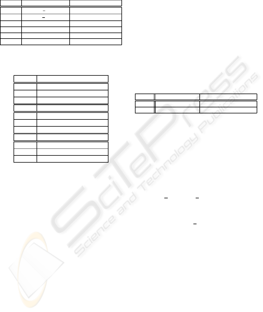
Table 1: Representations of the conformal geometric enti-
ties.
entity standard repr. direct repr.
Point P = x+
1
2
x
2
e
∞
+ e
0
Sphere s = P−
1
2
r
2
e
∞
s
∗
= x
1
∧ x
2
∧ x
3
∧ x
4
Plane π = n+de
∞
π
∗
= x
1
∧ x
2
∧ x
3
∧ e
∞
Circle z = s
1
∧ s
2
z
∗
= x
1
∧ x
2
∧ x
3
Line l = π
1
∧ π
1
l
∗
= x
1
∧ x
2
∧ e
∞
P-Pair P
p
= s
1
∧ s
2
∧ s
3
P
∗
p
= x
1
∧ x
2
Table 2: The geometric meaning of the inner product of
conformal vectorsU (1st column) andV (2nd column, rows
1,5, and 9).
U ·V plane
plane angle between planes
sphere Euclidean distance to center
point Euclidean distance
U ·V sphere
plane Euclidean distance to center
sphere distance measure
point distance measure
U ·V point
plane Euclidean distance
sphere distance measure
point Euclidean distance
dard representation a sphere is represented with the
help of its center point P and its radius r, while in
the direct representation it is constructed by the outer
product ’∧’ of four points x
i
that lie on the surface of
the sphere (x
1
∧ x
2
∧ x
3
∧ x
4
). In standard representa-
tion the dual meaning of the outer product is the in-
tersection of geometric entities. For example a circle
is defined by the intersection of two spheres (s
1
∧ s
2
).
Please notice that in this paper we indicate 3D vectors
by bold letters, e.g. n means the 3D normal vector of
a plane.
For the foundations of conformal geometric alge-
bra and its application to computer graphics refer for
instance to (L.Dorst et al., 2007), (Rosenhahn, 2003),
(Fontijne and Dorst, 2003) and to the tutorials (Dorst
and Mann, 2002), (Mann and Dorst, 2002), (Hilden-
brand et al., 2004) and (Hildenbrand, 2005).
3 DISTANCES AND ANGLES
In conformal geometric algebra distances and angles
are expressible easily with the help of the inner prod-
uct. Table 2 summarizes the geometric meaning of
the inner product of conformal vectors U and V.
The inner product of vectors in Conformal Geo-
metric Algebra results in a scalar and can be used as
a measure for distances between basic objects. The
inner product P· S of two vectors P and S can be used
for tasks like
• the Euclidean distance between two points
• the distance between one point and one plane
• the decision whether a point is inside or outside of
a sphere.
A vector in Conformal Geometric Algebra can be
written as
V = v
1
e
1
+ v
2
e
2
+ v
3
e
3
+ v
4
e
∞
+ v
5
e
0
(1)
The meaning of the two additional coordinates e
0
and
e
∞
is as follows :
v
5
= 0 v
5
6= 0
v
4
= 0 plane through origin sphere/point through origin
v
4
6= 0 plane sphere/point
The multiplication with a constant k 6= 0 leads al-
ways to the same geometric object (like in projective
space).
Division by v
5
6= 0 leads to (normalized form)
S = s
1
e
1
+ s
2
e
2
+ s
3
e
3
+ s
4
e
∞
+ e
0
(2)
representing a sphere S with center point s and ra-
dius r as
S = s+ s
4
e
∞
+ e
0
(3)
with
s
4
=
1
2
(s
2
− r
2
) =
1
2
(s
2
1
+ s
2
2
+ s
2
3
− r
2
)
Points are degenerate spheres with radius r = 0.
P = s+
1
2
s
2
e
∞
+ e
0
(4)
Planes are degenerate spheres with infinite radius.
They are represented as a vector with v
5
= 0
V = v
1
e
1
+ v
2
e
2
+ v
3
e
3
+ v
4
e
∞
= v + v
4
e
∞
(5)
The inner product of 3D vectors corresponds to the
well-known scalar product. The 3D basis vectors
e
1
,e
2
,e
3
square to 1
e
2
1
= e
2
2
= e
2
3
= 1 (6)
Because of the specific metric of the conformal space,
the additional basis vectors e
2
o
,e
2
∞
square to 0 and their
inner product results in e
∞
· e
o
= −1 . Based on these
specific properties the inner product between a Con-
formal vector U and a Conformal vector V is defined
by
U ·V = (u+ u
4
e
∞
+ u
5
e
o
) · (v+ v
4
e
∞
+ v
5
e
o
)
GRAPP 2008 - International Conference on Computer Graphics Theory and Applications
100

also expressible as
U ·V = u· v− u
5
v
4
− u
4
v
5
(7)
or
U ·V = u
1
v
1
+ u
2
v
2
+ u
3
v
3
− u
5
v
4
− u
4
v
5
In the case of U and V both being points we get
U ·V = −
1
2
(s− p)
2
We recognize that the square of the Euclidean dis-
tance of the inhomogenous points corresponds to the
inner product of the homogenous points multiplied by
−2.
(s− p)
2
= −2(U ·V) (8)
For a vectorU representing a point and a vectorV rep-
resenting a plane with normal vector n and distance d
we get according to equation (7)
U ·V = P· π = p· n− d (9)
representing the Euclidean distance of the point and
the plane. Note that the scalar product p· n describes
the distance of the plane from the origin. Subtraction
of d results in the Euclidean plane to point distance.
For a vector U representing a plane with normal vec-
tor n and origin distance d and a vectorV representing
a sphere we get according to equation (7)
U ·V = π · S = n· s− d (10)
representing the Euclidean distance of the sphere cen-
ter from the plane.
For two vectors S
1
and S
2
representing two spheres
we get
2(S
1
· S
2
) = r
2
1
+ r
2
2
− (s
2
− s
1
)
2
(11)
This means that twice the inner product of two
spheres equals the sum of the square of the radii mi-
nus the square of the Euclidean distance of the sphere
centers.
We will see now that the inner product of a point
and a sphere can be used for the decision of whether
a point is inside or outside of a sphere. For a vector
P representing a point (sphere with radius 0) and a
vector S representing a sphere with radius r we get
according to equation (11)
2(P· S) = r
2
− (s− p)
2
(12)
That is equal to the square of the radius minus the
square of the distance between the point and the
center point of the sphere.
Based on this observation we can see that for
P· S > 0 : p is inside of the sphere
P· S = 0 : p is on the sphere
P· S < 0 : p is outside of the sphere
Angles between two objects o
1
,o
2
like two lines
or two planes can be computed using the inner
product of the normalized direct representation of the
objects.
cos(θ) =
o
∗
1
· o
∗
2
o
∗
1
o
∗
2
(13)
or
θ = ∠(o
1
,o
2
) = arccos
o
∗
1
· o
∗
2
o
∗
1
o
∗
2
(14)
Please refer to (Doran and Lasenby, 2003) for more
details.
Let us derive as one example an expression for the
angle between two planes based on the observation of
equation (7). For a vector π
1
representing a plane with
normal vector n
1
and distance d
1
we get
u = n
1
, u
4
= d
1
, u
5
= 0
For a vector π
2
representing another plane we get
v = n
2
, v
4
= d
2
, v
5
= 0
The inner product of the two planes is
π
1
· π
2
= n
1
· n
2
(15)
representing the scalar product of the two normals of
the planes.
Based on this observation the angle θ between two
planes can be computed as follows
cos(θ) = π
1
· π
2
(16)
This corresponds to equation (14) taking into account
that the planes are normalized and that the dualization
operation only switches between the two possible an-
gles between planes.
Please notice that the same is also true for two cir-
cles. In this case the inner product describes the co-
sine of the respective carrier planes of the two circles.
4 DIFFERENTIAL GEOMETRY
In order to analyze point clouds some properties of
conformal geometric algebra are very helpful. As-
suming some kind of curvature information of point
clouds the easy handling of geometric objects like cir-
cles and lines can be used for the local description of
curvature. Based on these local properties the exis-
tence of geometric objects like cylinder, sphere, cone
or torus can be investigated.
(Adamson, 2007) already developed algorithms to
estimate local curvature information including princi-
pal curvatures. These can be very easily be transferred
into algebraic expressions describing locally fitting
objects. These objects include
ANALYSIS OF POINT CLOUDS - Using Conformal Geometric Algebra
101
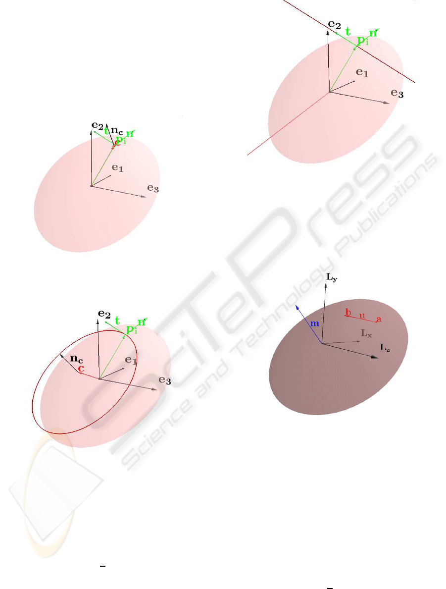
• osculating circle (see figure 2)
• line describing vanishing curvature (see figure 3)
• osculating circle with vanishing radius (see fig-
ure 1)
and can be treated very consistently in conformal geo-
metric algebra since all these objects have the same
algebraic structure. They are bivectors easy to com-
pute with.
Figure 1: Local coordinate system at point p
i
based on the
tangent vector t and the normal vector n.
Figure 2: Osculating circle describing the curvature at point
p
i
.
Circles can be described with the help of the outer
product of 3 points lying on the the circle or as the
intersection of a sphere and a plane resulting in the
following formula
Z = (c× n
c
)e
123
− n
c
∧ e
0
− (c· n
c
)e
∞
∧ e
0
+[(c· n
c
)c−
1
2
(c
2
− r
2
)n
c
] ∧ e
∞
Lines can be described with the help of the outer
product of 2 planes or as
L = ue
123
+ m∧ e
∞
(17)
Figure 3: Line describing vanishing curvature at point p
i
.
with u = b−a as Euclidean direction vector and m =
a × b as the moment vector. The corresponding six
Pl¨ucker coordinates are
(u : m) = (u
1
: u
2
: u
3
: m
1
: m
2
: m
3
). (18)
Figure 4: Pl¨ucker parameters u and m of the line through a
and b.
5 FITTING OF POINTS WITH
THE HELP OF A SPHERE
While in (Hildenbrand, 2005) fitting of spheres or
planes into point clouds is described, in this section
a point cloud p
i
∈ R
3
, i ∈ { 1,...,n} will be approxi-
mated specifically with the help of a sphere. The in-
homogenous points p
i
are represented as
P
i
= p
i
+
1
2
p
i
2
e
∞
+ e
0
(19)
and the sphere S with inhomogenous center point s
and radius r is represented according to equation (3).
GRAPP 2008 - International Conference on Computer Graphics Theory and Applications
102

5.1 Approach
In order to solve the approximation problem we
• define a distance measure between point and
sphere with the help of the inner product.
• make a least squares approach to minimize the
squares of the distances between the points and
the sphere.
• solve the resulting linear system of equations.
5.2 Distance Measure
According to section 3 the inner product between a
point P
i
and the sphere S
P
i
· S = (p
i
+
1
2
p
i
2
e
∞
+ e
0
) · (s+ s
4
e
∞
+ e
0
) (20)
can be used as a measure for their distance. This re-
sults in
P
i
· S = p
i
· s−
1
2
p
i
2
− s
4
according to equation (7) which can be written as
P
i
· S = w
i,1
s
1
+ w
i,2
s
2
+ w
i,3
s
3
+ w
i,4
s
4
+ w
i,5
or
P
i
· S =
4
∑
j=1
(w
i, j
s
j
) + w
i,5
(21)
with
w
i,k
=
p
i,k
: k ∈ {1, 2,3}
−1 : k = 4
−
1
2
p
i
2
: k = 5
5.3 Least Squares Approach
In the least-squares sense we consider the minimum
of the squares of the distances between all the points
and the sphere
min
n
∑
i=1
(P
i
· S)
2
(22)
In order to obtain the minimum we have the following
4 necessary conditions
∀k ∈ {1..4} :
∂(
∑
n
i=1
(P
i
· S)
2
)
∂s
k
=
n
∑
i=1
∂(P
i
· S)
2
∂s
k
= 0
(23)
With the help of
∂(P
i
· S)
2
∂s
k
= 2(P
i
· S) ·
∂(P
i
· S)
∂s
k
and
∂(P
i
· S)
∂s
k
=
∂(
∑
4
j=1
(w
i, j
s
j
) + w
i,5
)
∂s
k
= w
i,k
we obtain
∀k ∈ {1..4} :
n
∑
i=1
∂(P
i
· S)
2
∂s
k
= 2
n
∑
i=1
(
4
∑
j=1
(w
i, j
s
j
w
i,k
) + w
i,5
w
i,k
) = 0
or
∀k ∈ {1..4} :
n
∑
i=1
4
∑
j=1
(w
i, j
w
i,k
s
j
) = −
n
∑
i=1
(w
i,5
w
i,k
)
which is the same as
∀k ∈ {1..4} :
4
∑
j=1
n
∑
i=1
(w
i, j
w
i,k
s
j
) = −
n
∑
i=1
(w
i,5
w
i,k
)
or
∀k ∈ {1..4} :
4
∑
j=1
s
j
n
∑
i=1
(w
i, j
w
i,k
) = −
n
∑
i=1
(w
i,5
w
i,k
)
leading to the following linear equation system
∑
w
i,1
w
i,1
∑
w
i,2
w
i,1
∑
w
i,3
w
i,1
∑
w
i,4
w
i,1
∑
w
i,1
w
i,2
∑
w
i,2
w
i,2
∑
w
i,3
w
i,2
∑
w
i,4
w
i,2
∑
w
i,1
w
i,3
∑
w
i,2
w
i,3
∑
w
i,3
p
i,3
∑
w
i,4
w
i,3
∑
w
i,1
w
i,4
∑
w
i,2
w
i,4
∑
w
i,3
w
i,4
∑
w
i,4
w
i,4
· s
=
−
∑
w
i,5
w
i,1
−
∑
w
i,5
w
i,2
−
∑
w
i,5
w
i,3
−
∑
w
i,5
w
i,4
For a fitting sphere, the result of the least squares
approach is as follows :
∑
p
i,1
p
i,1
∑
p
i,2
p
i,1
∑
p
i,3
p
i,1
−
∑
p
i,1
∑
p
i,1
p
i,2
∑
p
i,2
p
i,2
∑
p
i,3
p
i,2
−
∑
p
i,2
∑
p
i,1
p
i,3
∑
p
i,2
p
i,3
∑
p
i,3
p
i,3
−
∑
p
i,3
−
∑
p
i,1
−
∑
p
i,2
−
∑
p
i,3
∑
1
· s
=
1
2
∑
p
i
2
p
i,1
1
2
∑
p
i
2
p
i,2
1
2
∑
p
i
2
p
i,3
−
1
2
∑
p
i
2
with p
i,1
, p
i,2
, p
i,3
as inhomogenous coordinatesof the
points p
i
. The result s = (s
1
,s
2
,s
3
,s
4
) represents the
center point of the sphere (s
1
,s
2
,s
3
) and its radius in
terms of r
2
= s
2
1
+ s
2
2
+ s
2
3
− 2s
4
6 BOUNDING SPHERE
ALGORITHM
The problem of defining a bounding sphere of a point
cloud can be subdivided into three sub-problems:
ANALYSIS OF POINT CLOUDS - Using Conformal Geometric Algebra
103
1. How to enclose a set of points by a minimal
sphere.
2. How to minimally expand an existing bounding
sphere when adding more points.
3. How to merge existing bounding spheres.
Because points can be treated as spheres of zero
radius, case 2 becomes part of case 3 if the latter is
solved for bounding sheres of general radii, including
the radius zero.
6.1 Point Clouds with One, Two or
Three Points
Conformal geometric algebra adds an origin-infinity
plane to 3D Eucldean space. The origin-infinity plane
is given by its bivector blade E = e
∞
∧ e
0
. The blade
E can be used to extract pure Euclidean parts from
conformal multivectors M
M
Euclid
= (M ∧ E) · E . (24)
We represent spheres by 5D vectors S in the
G
4,1
conformal model of three-dimensionalEuclidean
space. In general the conformal model uses blades A
V
for the socalled inner product null space representa-
tion (IPNS) of conformal subspaces V,
X · A
V
= 0 ⇔ X ∈ V, (25)
which is dual to the direct outer product null space
representation (OPNS)
X ∧A
∗
V
= 0 ⇔ X ∈ V, A
∗
V
= A
V
I
−1
5
= −A
V
e
123
E.
(26)
Section 2 gave examples of blades A
V
for circles and
lines and Equ. (29) shows how to obtain a sphere
(blade) vector (A
V
= S).
If the cloud consists of only one point
P = p+
1
2
p
2
e
∞
+ e
0
, (27)
this point defines its own bounding sphere with con-
formal center C = P and radius zero r = 0.
If the cloud consists of two points,
P
k
= p
k
+
1
2
p
2
k
e
∞
+ e
0
, 1 ≤ k ≤ 2, (28)
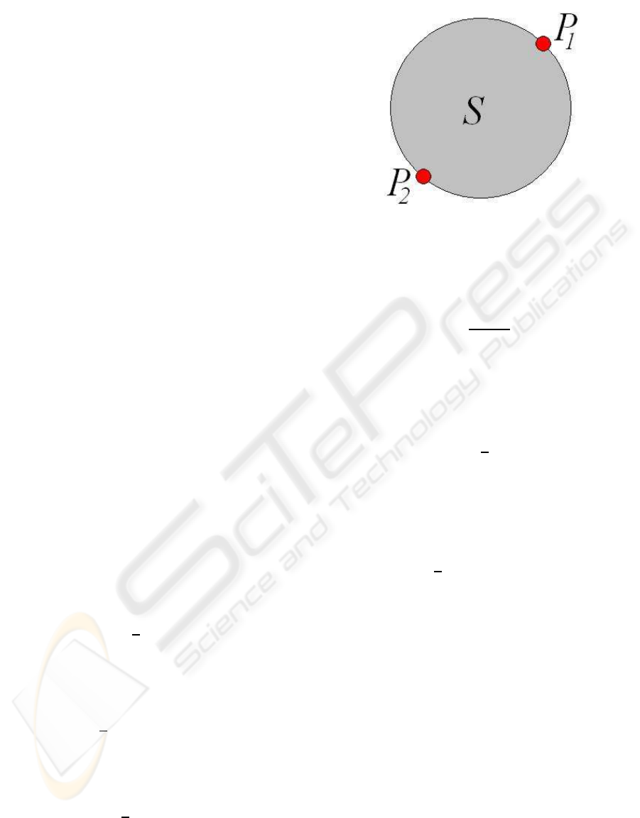
the minimal bounding sphere has P
1
and P
2
as its
poles. The conformal sphere vector (see Fig. 5) is
then given by
S =
1
2
(P
1
+ P
2
). (29)
The factor one half is convenient for keeping the
inner product of S with e
∞
to
S· e
∞
= −1. (30)
Figure 5: Sphere vector constructed from two pole points.
This is not necessary, because the conformal objects
are homogeneous, but helpful regarding numerical
implementations. We can always norm a sphere by
S →
S
−S· e
∞
(31)
and thus achieve (30). The radius of a normed sphere
is given by
r
2
= S
2
. (32)
The conformal center of a normed sphere is then given
by
C = S+
1
2
r
2
e
∞
. (33)
The Euclidean center vector of a sphere is given ac-
cording to (24) by
c = (C∧ E) · E. (34)
In the case of three conformal points
P
k
= p
k
+
1
2
p
2
k
e
∞
+ e
0
, 1 ≤ k ≤ 3, (35)
we can first define an initial sphere with two points
(e.g. P
1
,P
2
) as in Equ. (29). Then we can regard the
third point as a second sphere with zero radius and
center P
3
and apply the method for the bounding of
two spheres described in subsection 6.3. Or we can
directly expand the sphere to minimally include the
third point in the following way.
6.2 Minimally Including a New Point
We describe this alternative (compared to subsection
6.3) way in order to show that geometric algebra of-
fers a variety of algorithmic constructions, some of
which may be preferable for specific tasks and for nu-
merical optimization.
We show two variants in the form of CLUCalc
Scripts. The first more from a geometric algebra prin-
ciple point of view, the second based on further code
performance optimization with Maple.
GRAPP 2008 - International Conference on Computer Graphics Theory and Applications
104
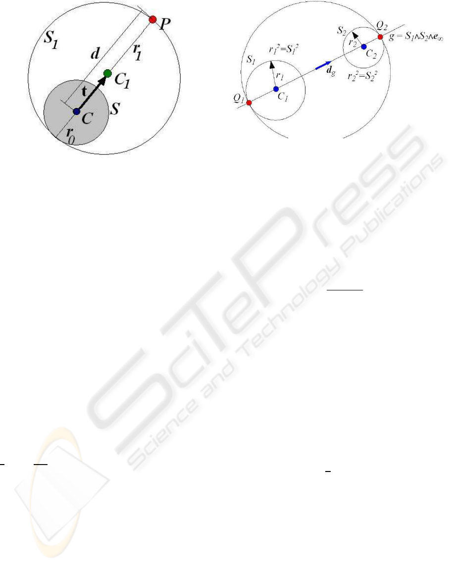
Figure 6: Minimally adding a point P to a sphere S by ad-
justing center and radius.
DefVarsN3(); // se of conformal model
:IPNS; // Use of inner product null space repr.
C = VecN3(c1,c2,c3); // Conformal sphere center
r=r0; // Sphere radius
S =C-0.5*r*r*einf;
//Definition of initial sphere S
P=VecN3(p1,p2,p3); // New point outside S
d = sqrt(-2*P.C);
//Distance between sphere center C and P
if (d>r){
CP = (p1-c1)*e1 + (p2-c2)*e2 + (p3-c3)*e3;
// Vector CP
T = 1 + 0.5* 0.5*(1-r/d)*CP *einf;
// Translator to new center
C1 = ˜T*C*T;
// Center of new sphere
r1 = (d+r)/2;
// Radius of new sphere
S1 = C1 - 0.5*r1*r1*einf;
// Def. of new sphere
}
We see in the CLUCalc Script that the sphere is
only expanded if the new point P is outside the sphere
S (d > r). C
1
is the center of the expanded sphere S
1
,
obtained by shifting C in the direction of P by t =
1
2
(d − r)
CP
|CP|
, because d = |CP|. r
1
= (d + r)/2 is the
radius of the minimally expandedsphere S
1
. Compare
Fig. 6.
For numerical optimization we can replace the
definition of d and the if loop by Maple optimized
code
d=sqrt((p1-c1)*(p1-c1)+(p2-c2)*(p2-c2)+(p3-c3)*(p3-c3));
if (d>r){
c1x = (-r*p1+r*c1+p1*d+c1*d)/d/2;
c1y = ( r*c2+p2*d+c2*d-r*p2)/d/2;
c1z = ( p3*d-r*p3+r*c3+c3*d)/d/2;
r1 = (d+r)/2;
S1 = VecN3(c1x,c1y,c1z) - 0.5*r1*r1*einf;}
Figure 7: Minimal bounding sphere of two spheres.
6.3 Bounding Two Spheres
We can merge (bound) two spheres by defining a
straight line g which connects the centers of the two
(normed) spheres S
1
and S
2
g
∗
= (S
1
∧ S
2
∧ e
∞
)
∗
. (36)
The Eulidean unit vector in the direction of g is then
d =
g
∗
· e
123
|g
∗
· e
123
|
. (37)
We now calculate the poles of the minimal bounding
sphere. The first pole is the point of intersection of g
with S
1
away from S
2
q
1
= c
1
− r
1
d, (38)
with c
1
and r
1
calculated according to (34) and (32).
We similarly obtain the second pole of the bounding
sphere as the point of intersection of g with S
2
away
from S
1
q
2
= c
2
+ r
2
d, (39)
The corresponding conformal poles (27) give accord-
ing to (29) the mininal bounding sphere (see Fig. 7)
S
12
=
1
2
(Q
1
+ Q
2
). (40)
In this section we developed the algebraic expres-
sions for the minimal bounding sphere [eqs. (36) to
(40)] for easy numerical implementation. It would be
possible to completely carry out the calculation of S
12
on the conformal level. For that purpose we would
first calculate the conformal point pairs (OPNS) of in-
tersection of line g with sphere S
1
pair
1
= g · S
1
(41)
and of line g with sphere S
2
pair
2
= g · S
2
. (42)
ANALYSIS OF POINT CLOUDS - Using Conformal Geometric Algebra
105

With
Q
1
=
pair
1
+ |pair
1
|
pair
1
· e
∞
(43)
and
Q
2
=
pair
2
− |pair
2
|
pair
2
· e
∞
(44)
we can then directly pick the conformal points Q
1
and
Q
2
out of the point pairs pair
1
and pair
2
.
If (like in subsection 6.2) the second sphere S
2
happens to be only a point (sphere with zero radius),
we can omit the calculation of Q
2
in Equs. (39), (42)
and (44). We simply replace Q
2
= S
2
in Equ. (40).
6.4 Comparison with Welzl’s Bounding
Sphere Algorithm
The iteration of the method suggested in subsection
6.3 (test of inclusion, and if necessary the calcula-
tion of the new bounding sphere) results in the final
bounding sphere of n points in linear time O(n). The
proposed method is easy to understand and with given
routines for inner and outer products easy to imple-
ment. As demonstrated in subsection 6.2 the algo-
rithm can be further optimized with Maple. In aver-
age Welzl’s algorithm (Welzl, 1991) also runs in as-
ymptotically linear time, but the recursion in Welzl’s
algorithm makes it harder to examine and guarantee
the performance time.
7 CONCLUSIONS
We presented a bunch of basics and algorithms ex-
pressed in the mathematical framework of conformal
geometric algebra. We are convinced that its easy
handling of geometric objects like spheres, circles or
planes, its easy handling of distances and angles be-
tween them as well as its way of fitting and bounding
of geometric objects will provide a promising foun-
dation for the analysis of point clouds.
REFERENCES
Adamson, A. (2007). Computing Curves and Surfaces from
Points. PhD thesis, Darmstadt University of Technol-
ogy.
Doran, C. and Lasenby, A. (2003). Geometric Algebra for
Physicists. Cambridge University Press.
Dorst, L. and Mann, S. (2002). Geometric algebra: a
computational framework for geometrical applica-
tions (part i: algebra). Computer Graphics and Ap-
plication, 22(3):24–31.
Fontijne, D. and Dorst, L. (2003). Modeling 3D euclid-
ean geometry. IEEE Computer Graphics and Appli-
cations, 23(2):68–78.
Hildenbrand, D. (2005). Geometric computing in computer
graphics using conformal geometric algebra. Comput-
ers & Graphics, 29(5):802–810.
Hildenbrand, D., Fontijne, D., Perwass, C., and Dorst, L.
(2004). Tutorial geometric algebra and its applica-
tion to computer graphics. In Eurographics confer-
ence Grenoble.
Hildenbrand, D., Fontijne, D., Wang, Y., Alexa, M., and
Dorst, L. (2006). Competitive runtime performance
for inverse kinematics algorithms using conformal
geometric algebra. In Eurographics conference Vi-
enna.
L.Dorst, Fontijne, D., Mann, S., and Kaufman, M. (2007).
Geometric Algebra for Computer Science, An Object-
Oriented Approach to Geometry. Morgan Kaufman.
Mann, S. and Dorst, L. (2002). Geometric algebra: a
computational framework for geometrical applica-
tions (part ii: applications). Computer Graphics and
Application, 22(4):58–67.
Rosenhahn, B. (2003). Pose Estimation Revisited. PhD
thesis, Inst. f. Informatik u. Prakt. Mathematik der
Christian-Albrechts-Universit¨at zu Kiel.
Schnabel, R., Wahl, R., and Klein, R. (2007). Efficient
ransac for point-cloud shape detection. Computer
Graphics Forum, 26(2):214–226.
Welzl, E. (1991). Smallest enclosing disks (balls and ellip-
soids. In Lecture Notes in Computer Science, pages
555:359–370.
GRAPP 2008 - International Conference on Computer Graphics Theory and Applications
106
