
APPROXIMATE G
1
CUBIC SURFACES FOR DATA
APPROXIMATION
Yingbin Liu and Stephen Mann
University of Waterloo, Waterloo, Ontario, Canada
Keywords:
CAGD, Triangular B
´
ezier patches, Continuity.
Abstract:
This paper presents a piecewise cubic approximation method with approximate G
1
continuity. For a given
triangular mesh of points with arbitrary topology, one cubic triangular B
´
ezier patch surface is constructed.
The resulting surfaces have G
1
continuity at the vertex points, but only requires approximate G
1
continuity
along the macro-patch boundaries so as to lower the patch degree. While our scheme cannot generate the
surfaces in as high quality as Loop’s sextic scheme, they are of half the polynomial degree, and of far better
shape quality than the results of interpolating split domain schemes.
1 INTRODUCTION
In computer graphics applications, a surface is usually
constructed from a given data set that represents more
or less precisely the surface shape. Due to their el-
egant geometric properties, triangular B
´
ezier patches
are often used to interpolate or approximate a triangu-
lated data mesh. The main difficulty to interpolate or
approximate a given data mesh is how to satisfy the
restrictions imposed on the control points to obtain
surface patches that meet with a given order of conti-
nuity. In most cases, we want the surface patches to
be visually smooth and meet with G
1
continuity.
In past work, different G
1
schemes using domain
splits were devised to fit multiple patches (three or
four) to each data triangle (Peters, 1990; Piper, 1987;
Shirman and S
´
equin, 1991; Hahmann and Bonneau,
2003; Mann et al., 1992). Since it is impossible to
generated G
1
continuous surfaces on arbitrary data
sets using cubic patches (Piper, 1987; Peters, 1990),
these schemes use at least quartic patches to guar-
antee G
1
continuity along the macro-patch bound-
aries. It was later shown that the results from these
local interpolation schemes do not generate satisfac-
tory shapes (Mann et al., 1992). Loop designed a
scheme using sextic triangular B
´
ezier patches in one-
to-one correspondence with the data triangles (Loop,
1994). In Loop’s scheme, an approximation method
using transformed data vertices was also presented to
create smooth surfaces with high quality. In all these
schemes, control points are set to meet the constraints
required by G
1
continuity along the patch boundaries.
The price to fulfil the G
1
constraints is that we have
to use high degree (at least quartic) and/or multiple
patches and possibly sacrifice shape quality.
Approximate G
1
continuity is a relaxation of G
1
continuity where patches meet C
0
but the discontinu-
ity in the surface normals between adjacent patches
is small. Previous work on approximate G
1
construc-
tions includes parametric interpolation of positions,
normals, and second fundamental forms at the data
points (Mann, 1992); interpolations with cubic preci-
sion on positions and normals at the data points, both
in the functional case (Liu and Mann, 2005) and the
parametric case (Liu and Mann, 2007). In this paper,
the given data network is approximated by integrat-
ing techniques from Loop’s scheme to construct the
boundary curves (Loop, 1994). For each data triangle,
three cubic triangular patches are created to meet with
C
1
continuity. As for the macro-boundaries, i.e., the
boundaries between patches from different data trian-
gles, since we only require approximate G
1
continu-
ity, some discontinuity exists in the surface normals.
To decrease this normal discontinuity, two neighbour-
ing patches across the macro-patch boundaries are ad-
justed later to have equal normals at the middle point
39
Liu Y. and Mann S. (2008).
APPROXIMATE G1 CUBIC SURFACES FOR DATA APPROXIMATION.
In Proceedings of the Third International Conference on Computer Graphics Theory and Applications, pages 39-44
DOI: 10.5220/0001093400390044
Copyright
c
SciTePress
on the common boundary curve.
The remaining parts of this paper are arranged as
follows: Section 2 reviews the G
1
continuity con-
straints; the details of our approximation is introduced
in Section 3; in Section 4, we show some resulting
surfaces, which we compare to surfaces generated by
other G
1
schemes; conclusions and possible future
work are presented in Section 5.
2 CONTINUITY CONSTRAINTS
A triangular B
´
ezier patch of degree n is defined as
S(u, v,w) =
∑
i+ j+k=n
P
i jk
B
n
i jk
(u,v,w).
Here (u,v,w) are barycentric coordinates for the para-
meter; B
n
i jk
(u,v,w) is the generalized Bernstein poly-
nomial; P
i jk
are the control points of the patch. For
two triangular patches to join each other with G
1
con-
tinuity, i.e., the tangent planes from the two adjacent
patches are coplanar at any point along the boundary
curve, certain constraints must be fulfilled.
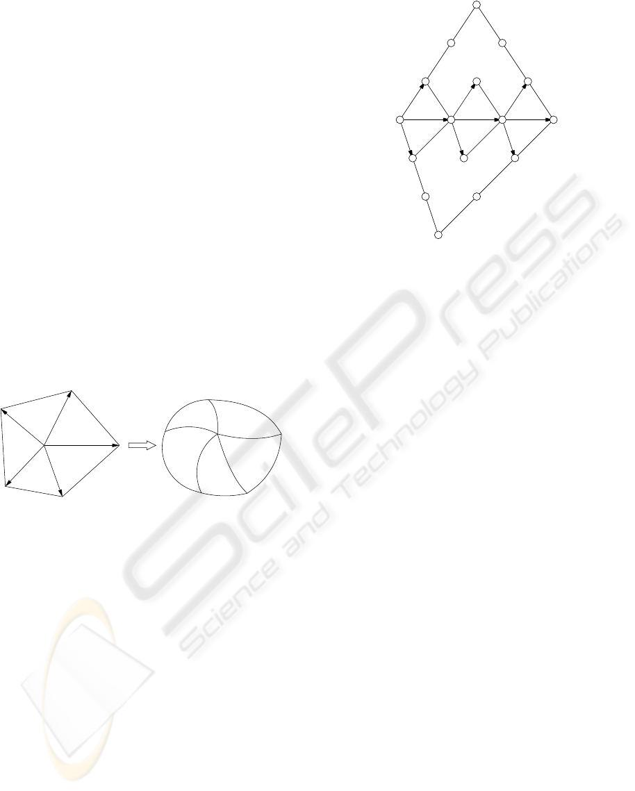
H
i
V
V
i
F
i−1
F
i
Figure 1: G
1
continuity at a vertex.
For a vertex V with valence n in our mesh, we num-
ber the surrounding patches F
i
, i = 0, . ..,n − 1, in
anti-clockwise order. Figure 1, right, shows a pair
of neighbouring patches F
i−1
and F
i
with common
boundary H
i
, with their domain triangles appearing
on the left of the figure. The parametric direction for
the partial derivative along the common edge is de-
fined from V to V
i
in the domain triangles.
In this paper, we focus on cubic B
´
ezier patches to
explore the G
1
continuity conditions. Two adjacent
cubic patches F
i
and F
i−1
with their control points are
shown in Figure 2. We define the following vectors:
~u
j
= H
j+1
i
− H
j
i
, ~v
j
= F
j
i
− H
j
i
, ~w
j
= F
j
i−1
− H
j
i
,
with j = 0, 1,2. Then for any given point along the
boundary curve, the tangent planes calculated from
the two patches are defined by vectors ~u, ~v and ~w, all
of which are quadratic B
´
ezier functions:
~u =
2
∑
j=0
~u
j
B
n
j
(t), ~v =
2
∑
j=0
~v
j
B
n
j
(t), ~w =
2
∑
j=0
~w
j
B
n
j
(t).
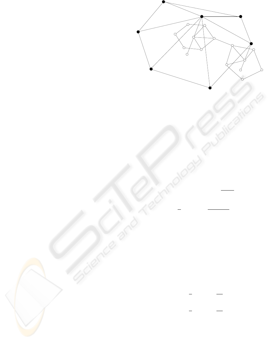
H
3
i
F
0
i
F
1
i
F
1
i−1
F
2
i−1
H
0
i
F
0
i−1
H
1
i
H
2
i
F
2
i
Figure 2: Adjacent cubic patches.
If patches F
i
and F
i−1
meet with G
1
continuity, they
must share the control points of the common bound-
ary H
j
i
, j = 0,1, 2, 3. Moreover, the two tangent
planes at any boundary point should be coplanar, i.e.,
there exist scalar valued functions φ(t), µ(t) and ν(t)
such that for any parameter value t, t ∈ [0,1], we have
φ(t)~u = µ(t)~v + ν(t)~w. (1)
To guarantee the proper orientation of the tangents,
assume µ(t)ν(t) ≥ 0. Since it is not guaranteed to
create surface using cubic patches to have G
1
con-
tinuity (Piper, 1987; Peters, 1990), all the existing
G
1
schemes use at least quartic patches (Shirman and
S
´
equin, 1991; Mann et al., 1992)
For all the patches to meet with G
1
continuity at
vertex V , the G
1
constraints of Equation 1 are applied
to all boundaries originating from vertex V . Differen-
tiating these equations and evaluate at vertex V results
in a linear system. Solving this system is called the
“twist compatibility” or “vertex consistency” prob-
lem, and it has been shown that this linear system may
not have a solution (Watkins, 1988; Sarraga, 1988;
Loop, 1994). Even if there exists a G
1
solution by
solving the twist compatibility problem, it is not clear
that the resulting surface has a satisfactory shape.
In the past work, one approach to construct G
1
continuous surfaces is to perform a Clough-Tocher
like domain split on each patch F
i
surrounding vertex
V (Clough and Tocher, 1965). At least quartic degree
patches are used in a domain split method (Shirman
and S
´
equin, 1991). Alternatively, Loop invented a so-
lution to solve the twist compatibility using one sextic
patch for each data triangle (Loop, 1994), with details
introduced in Section 3.1.
Instead of using high degree patches to fulfil the
G
1
constraints, we focus on using low degree (cu-
bic) patches to create surfaces with approximate G
1
GRAPP 2008 - International Conference on Computer Graphics Theory and Applications
40
continuity. With the approximate G
1
method, we al-
low a small amount of normal discontinuity across the
boundary curves. However, we still require G
1
conti-
nuity at the vertex points to keep the surface disconti-
nuity going too high. Using the freedom provided by
this relaxation, the goals of our method include:
• Use of cubic patches,
• Better shaped surfaces.
3 CUBIC APPROXIMATION
The goal of our work is to approximate the shape rep-
resented by a given data mesh as accurately as pos-
sible, but using lower degree patches than the G
1
schemes. We achieve this reduction in degree by
only requiring approximate G
1
continuity along patch
boundaries. In the cubic scheme we describe in this
paper, we construct the surface by creating boundary
curves for each edge of a data triangle, and then per-
form a Clough-Tocher like domain split on the cubic
patch. After the interior of the patches is filled, we
then do some adjustments to lower the normal dis-
continuity along the boundaries.
3.1 Loop’s Scheme
In Loop’s scheme, boundary curves are constructed
so that the solutions for the twist terms are guaran-
teed (Loop, 1994). Loop’s sextic scheme has the fol-
lowing steps:
1. Construct quartic boundary curves.
2. Solve the twist terms.
3. Construct tangent fields along the boundaries.
4. Elevate the degree of the boundary curves to sex-
tic.
5. Set the second row of control points in the sextic
patch to interpolate the tangent fields.
6. Set the remaining center control point by averag-
ing the control points from above steps.
When the valences of the three vertices of a data trian-
gle are equal, the patch constructed by Loop’s scheme
is quintic; if the three valences are all six, then the
patch degree reduces to quartic (Loop, 1994). Our
cubic scheme integrated the boundary tangents con-
struction from the first step in Loop’s scheme, but
generating cubic boundary curves.
H
1
i
A
H
0
i
V
i+1
V
V
i
H
1
i−1
H
1
i+1
V
i−1
H
2
i
H
3
i
Figure 3: Construction of boundary curves.
3.2 Boundary Construction
For the edge between the vertex V and its neighbour
V
i
, we use some ideas of Loop (Loop, 1994) to con-
struct a cubic boundary curve H
i
, as illustrated in Fig-
ure 3. Since the curve is cubic, there are four control
points: H
0
i
, H
1
i
, H
2
i
, H
3
i
to be constructed. For the ver-
tex V , the control points H
0
i
and H
1
i
are constructed as
H
0
i
= αV + (1 − α)A = αV +
1 − α
n
n−1
∑
k=0
V
k
, (2)
H
1
i
= H
0
i
+
β
n
n−1
∑
k=0
cos
2(k − i)π
n
V
k
. (3)
Here n is the valence of the vertex V ; point A is the
average of all neighbours of vertex V ; α and β are two
shape parameters. When α = 1, the resulting surface
interpolates the data vertices, shown as V
i
in Figure 3.
For α to be other values, the resulting surface approx-
imates the given data mesh. Parameter β defines the
length of the tangent vector at H
0
i
. In our cubic ap-
proximation scheme, the α and β are set with an ex-
perimental value the same as in Loop’s scheme:
α =
1
9
4 + cos(
2π
n
)
,
β =
1
3
1 + cos(
2π
n
)
. (4)
With this α value, our scheme does not interpolate the
given data vertices, but generating an surface approx-
imating the shape of the given data mesh.
The construction of control points H
0
i
and H
1
i
performs a first order Fourier transformation on all
the neighbouring vertices of V (Loop, 1994; Davis,
1979). If all the control points H
1
i
are connected,
they form a regular n-gon with H
0
i
being the centre,
APPROXIMATE G1 CUBIC SURFACES FOR DATA APPROXIMATION
41
as shown in the Figure 3. Point H
0
i
is the affine com-
bination of the data vertex V and the average center of
V ’s neighbours, and all the boundary curves connect-
ing V share the same position of point H
0
i
. The other
two control points H
2
i
and H
3
i
are calculated similarly
with Equation 3, using the information of V
i
’s neigh-
bours.
In Loop’s scheme, quartic boundary curves have
to be used to fulfil the strict G
1
continuity conditions,
and later the patch degree is elevated to sextic for the
same reason.
3.3 Patch Construction
Past work shows that it can be impossible to gener-
ate G
1
continuous surfaces using cubic patches (Piper,
1987; Peters, 1990). When using approximate G
1
continuity, we found there was insufficient degrees of
freedom if we only used one cubic patch per data tri-
angle. In particular, with one cubic patch per face,
since the center control point of this patch affects the
normals along all three boundaries, it is difficulty to
place this control point to yield surfaces with accept-
able smoothness. To improve surface smoothness and
still use cubics, we perform a Clough-Tocher like do-
main split (Clough and Tocher, 1965) to construct
three micro-patches for each data triangle.
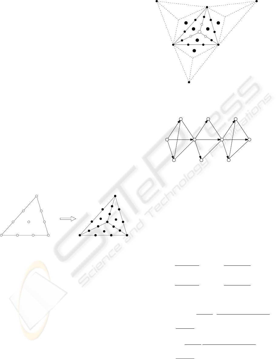
Figure 4: Macro patch split.
We first construct one cubic patch for each data trian-
gle, as shown on the left in Figure 4. The boundaries
of this initial patch are set with the methods described
in Section 3.2. We set the center control point to be
the weighted average of the other nine control points,
using a method similar to the way introduced in one
author’s previous paper (Mann, 1999).
We then subdivide the patch into three cubic
patches (called micro patches), as shown in the right
of Figure 4. The subdivided control points are shown
as small black dots in Figure 5. The small white and
the big white points are constructed as the gravity cen-
tre of the adjacent three control points, as in Clough-
Tocher’s scheme (Clough and Tocher, 1965; Farin,
1986; Mann, 1999). After the split, the center control
point of each micro-patch, shown as big black dots in
Figure 5, only affects the continuity along the corre-
sponding macro-patch boundary. The initial positions
Figure 5: Control points construction.
F
0
i
F
1
i
F
2
i
F
0
i−1
F
1
i−1
F
2
i−1
H
3
i
H
0
i
H
1
i
H
2
i
P
0
P
2
Figure 6: Ratios of intersection.
for these three points are set by local averaging. As
shown in Figure 6, The two pairs of side panels are
set to be coplanar to have equal normals at end data
points H
0
i
and H
3
i
. Let F
0
i
F
0
i−1
intersect H
0
i
H
1
i
at P
0
,
F
2
i
F
2
i−1
intersect H
2
i
H
3
i
at P
2
, as shown in Figure 6.
Here the points F
j
i
and F
j
i−1
( j = 0, 1, 2) are the micro
patch control points resulting from the Clough-Tocher
like split. The ratios of the intersection are then de-
fined as
η
0
=
|P
0
− H
0
i
|
|H
1
i
− H
0
i
|
, γ
0
=
|F
0
i−1
− P
0
|
|F
0
i−1
− F
0
i
|
,
η
2
=
|P
2
− H
2
i
|
|H
3
i
− H
2
i
|
, γ
2
=
|F
2
i−1
− P
2
|
|F
2
i−1
− F
2
i
|
.
We set the initial position for point F
1
i
and F
1
i−1
as
F
1
i
= H
1
i
+ (1 −
γ
0
+ γ
2
2
)
F
0
i
− F
0
i−1
+ F
2
i
− F
2
i−1
2
+
η
0
+ η
2
2
(H
2
i
− H
1
i
),
F
1
i−1
= H
1
i
−
γ
0
+ γ
2
2
F
0
i
− F
0
i−1
+ F
2
i
− F
2
i−1
2
+
η
0
+ η
2
2
(H
2
i
− H
1
i
). (5)
The two center control points across the macro-
patch boundary are then adjusted by adding an offset
GRAPP 2008 - International Conference on Computer Graphics Theory and Applications
42
vector that is calculated with the method introduced in
our previous paper. After the adjustments, the normal
vectors of two patches at the middle boundary point is
equal. Theoretically, we can adjust the center points
to have equal normals at two or three points along the
boundary, but that will make the scheme not stable. In
all the examples shown in Section 4, all the surfaces
by our scheme have equal normals only at one middle
boundary points.
This cubic scheme is approximately G
1
along the
macro-patch boundaries, although patches meet with
G
1
continuity at the vertex points; the patches meet
with C
1
continuity along the boundaries between two
micro-patches; and the three micro-patches meet with
C
2
at the split point, a result of the averaging in Step
3 of (Farin, 1986).
4 RESULTS
We compared the resulting surfaces of our cubic
scheme to those generated by Loop’s scheme, with
both the interpolation and the approximation results.
Since Loop’s scheme does not use the domain split
method, we also generated surfaces on the same
models using Shirman-S
´
equin’s quartic scheme to
make the comparison more comprehensive. Shirman-
S
´
equin’s scheme generates surfaces with data vertices
interpolated, and it also performs a domain split sim-
ilar to Clough-Tocher’s (Shirman and S
´
equin, 1991).
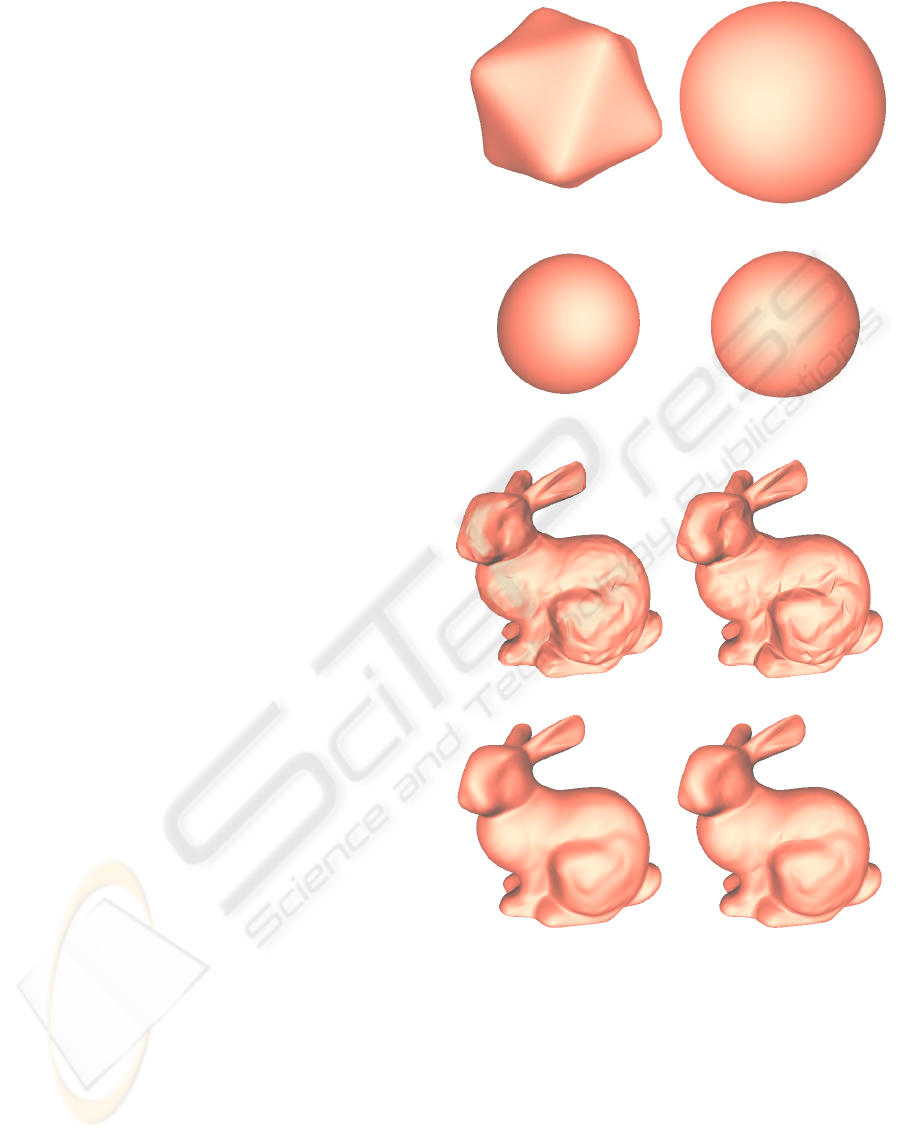
In Figure 7, we show four surfaces fit to an icosa-
hedron. The top left is Loop’s interpolating sur-
face; the bottom left is Loop’s approximating surface;
the top right is the quartic, G
1
scheme by Shirman-
S
´
equin; the bottom right is our cubic, approximate G
1
scheme. Loop’s approximate scheme has much bet-
ter shape than his interpolating scheme; our cubic ap-
proximation scheme has similar shape to Loop’s. The
highest normal discontinuity is 0.48 degree on our cu-
bic surface.
In Figure 8, we show four surfaces fitted to the
Stanford bunny model. The order of the schemes is
the same as in Figure 7. While the two interpolat-
ing schemes show numerous shape artifacts, both ap-
proximating schemes produce surfaces with far bet-
ter shape quality. In this model, the highest normal
discontinuity is 19.57 degree for our cubic surface.
However, boundaries with high normal discontinuity
angles (more than 10 degrees) account for about 0.8%
of all boundary curves. While some artifacts are visi-
ble in our approximate G
1
scheme, we see substantial
improvement over the similar interpolating scheme.
Figure 7: Icosahedron surfaces.
Figure 8: Bunny surfaces.
5 CONCLUSIONS
In this paper we presented a cubic approximating
scheme to generate surfaces characterizing the shape
of given data mesh with low price. Although the nor-
mal discontinuities on the resulting surfaces are visi-
ble on some test models, the overall surface shape is
good. Further, our scheme is only cubic and it will of-
fer great advantage for easy implementation and sta-
bility.
APPROXIMATE G1 CUBIC SURFACES FOR DATA APPROXIMATION
43

In the future, we will do further analysis on the
cross boundary discontinuity, and derive an upper
bound for it. We will also look for methods to guar-
antee that the normal discontinuity does not exceed
a specified bound. This will likely result in condi-
tions similar to the vertex consistency conditions, but
our expectation is that we will be able to trade patch
shape for lower normal discontinuity.
REFERENCES
Clough, R. and Tocher, J. (196 5). Finite element stiffness
matrices for analysis of plates in bending. In Proceed-
ings of Conference on Matrix Methods in Structural
Analysis.
Davis, P. (1979). Circulant Matrices. Wiley, New York.
Farin, G. (1986). Triangular Berstein-B
´
ezier patches. Com-
puter Aided Geometric Design, 3(2):83–127.
Hahmann, S. and Bonneau, G.-P. (2003). Polynomial
surfaces interpolating arbitrary triangulations. IEEE
Transactions on Visualization and Computer Graph-
ics (TVCG), 9(1):99–109.
Liu, Y. and Mann, S. (2005). Approximate continu-
ity for functional, triangular B
´
ezier patches. SIAM-
Geometric Modeling 2005.
Liu, Y. and Mann, S. (2007). Approximate continuity for
parametric b
´
ezier patches. ACM Solid and Physical
Modeling Symposium.
Loop, C. (1994). A G
1
triangular spline surface of arbitrary
topological type. Computer Aided Geometric Design,
11(3):303–330.
Mann, S. (1992). Surface Approximation Using Geometric
Hermite Patches. PhD thesis, University of Washing-
ton.
Mann, S. (1999). Cubic precision clough-tocher interpola-
tion. Computer Aided Geometric Design, 16(2):85–
88.
Mann, S., Lounsbery, M., Loop, C., Meyers, D., Painter, J.,
DeRose, T., and Sloan, K. (1992). Curve and Surface
Design, Chapter 8, A Survey of Parametric Scattered
Data Fitting Using Triangular Interpolants. SIAM.
Peters, J. (1990). Smooth mesh interpolation with cubic
patches. Computer-aided Design, 22/2:109–120.
Piper, B. P. (1987). Visually smooth interpolation with tri-
angular b
´
ezier patches. In Farin, G., editor, Geometric
Modeling: Algorithms and New Trends, pages 221–
234. SIAM.
Sarraga, R. F. (1988). G
1
interpolation of generally unre-
stricted cubic b
´
ezier curves. Computer Aided Geo-
metric Design, 4(1-2):23–40.
Shirman, L. and S
´
equin, C. (1991). Local surface interpo-
lation with b
´
ezier patches: Errata and improvements.
Computer Aided Geometric Design, 8(3):217–221.
Watkins, M. A. (1988). Problems in geometric continuity.
Computer Aided Geometric Design, 20(8):499–502.
GRAPP 2008 - International Conference on Computer Graphics Theory and Applications
44
